Load libraries
library(psych)
library(tidyverse)
library(lavaan)
library(semTools)
library(manymome)Principles and Practice of Structural Equation Modeling (5e) by Rex B. Kline
library(psych)
library(tidyverse)
library(lavaan)
library(semTools)
library(manymome)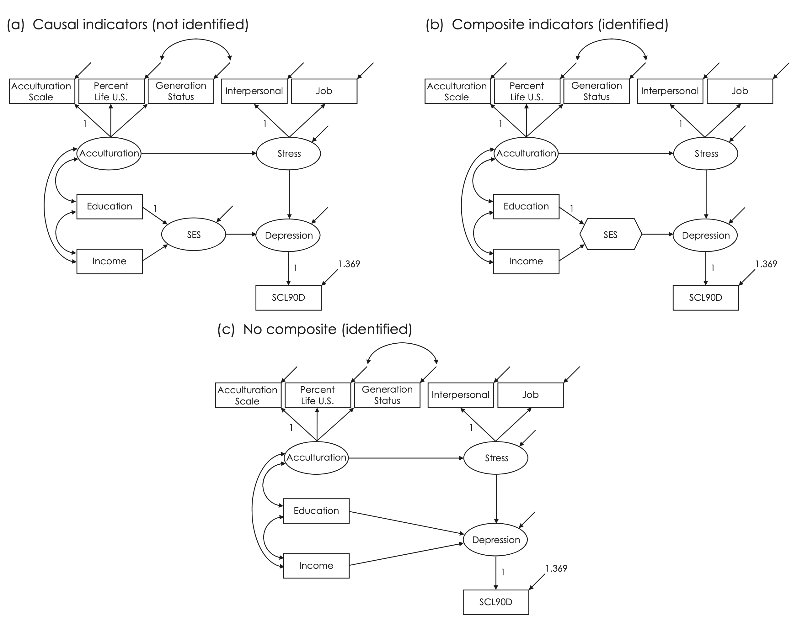
FIGURE 16.2. Structural regression models with causal indicators for a latent socioeconomic status composite with a disturbance (a). Zero‐error variance model with composite indicators for an SES composite with no disturbance (b). A partially reduced form model with no SES composite (c). Model (a) is not identified, models (b) and (c) are equivalent. (p. 292)
# input the correlations in lower diagnonal form
shenLower.cor <- '
1.00
 .44 1.00
 .69  .54 1.00
 .21  .08  .16 1.00
 .23  .15  .19  .19 1.00
 .12  .08  .08  .08 -.03 1.00
 .09  .06  .04  .01 -.02  .38 1.00
 .03  .02 -.02 -.07 -.11  .37  .46 1.00 '

# name the variables and convert to full correlation matrix
shen.cor <- lavaan::getCov(shenLower.cor, names = c("acculscl", "status",
 "percent", "educ", "income", "interpers", "job", "scl90d"))

# add the standard deviations and convert to covariances
shen.cov <- cor2cov(shen.cor, sds = c(3.60,3.30,2.45,3.27,3.44,2.99,
 3.58,3.70))
# display correlations and covariances
shen.cor |> print() acculscl status percent educ income interpers job scl90d
acculscl 1.00 0.44 0.69 0.21 0.23 0.12 0.09 0.03
status 0.44 1.00 0.54 0.08 0.15 0.08 0.06 0.02
percent 0.69 0.54 1.00 0.16 0.19 0.08 0.04 -0.02
educ 0.21 0.08 0.16 1.00 0.19 0.08 0.01 -0.07
income 0.23 0.15 0.19 0.19 1.00 -0.03 -0.02 -0.11
interpers 0.12 0.08 0.08 0.08 -0.03 1.00 0.38 0.37
job 0.09 0.06 0.04 0.01 -0.02 0.38 1.00 0.46
scl90d 0.03 0.02 -0.02 -0.07 -0.11 0.37 0.46 1.00shen.cov |> round(2) |> print() acculscl status percent educ income interpers job scl90d
acculscl 12.96 5.23 6.09 2.47 2.85 1.29 1.16 0.40
status 5.23 10.89 4.37 0.86 1.70 0.79 0.71 0.24
percent 6.09 4.37 6.00 1.28 1.60 0.59 0.35 -0.18
educ 2.47 0.86 1.28 10.69 2.14 0.78 0.12 -0.85
income 2.85 1.70 1.60 2.14 11.83 -0.31 -0.25 -1.40
interpers 1.29 0.79 0.59 0.78 -0.31 8.94 4.07 4.09
job 1.16 0.71 0.35 0.12 -0.25 4.07 12.82 6.09
scl90d 0.40 0.24 -0.18 -0.85 -1.40 4.09 6.09 13.69zero error variance model
# ses with composite indicators (educ, income)
# educ, income each covary with acculturation factor

# special lavaan syntax for composite indicators
# "<~" defines a composite where the disturbance
# variance is automatically fixed to zero
# composite is explicitly scaled with an ULI constraint

shenSEScomposite.model <- '
# ses composite
 SES <~ 1*educ + income

# reflective factors
 Acculturation =~ acculscl + status + percent
 status ~~ percent
 Stress =~ interpers + job
 Depression =~ scl90d
 scl90d ~~ 1.369*scl90d

# covariances among exogenous acculturation factor
# and composite indicators of ses explicitly defined
# as free parameters
 Acculturation ~~ income + educ
 income ~~ educ

# covariance between ses composite and acculturation
# factor fixed to zero
 Acculturation ~~ 0*SES

# structural model
 Stress ~ Acculturation

# depression regressed on ses composite and
# reflective stress factor
# coefficient for SES labeled for calculation of
# indirect effects through the SES composite
Depression ~ b*SES + Stress 'partially reduced form model with no SES composite
# specify figure 16.2(c)
# partially reduced form model with
# no SES composite

shenSESnoComposite.model <- "
  # reflective factors
  Acculturation =~ acculscl + status + percent
  status ~~ percent
  Stress =~ interpers + job
  Depression =~ scl90d
  scl90d ~~ 1.369*scl90d

  # covariances among exogenous acculturation factor
  # and the measured exogenous variables income and education
  # explicitly declared as free parameters
  Acculturation ~~ income + educ
  income ~~ educ

  # structural model
  Stress ~ Acculturation

  # depression regressed on income, educ, and
  # reflective stress factor
  Depression ~ educ + income + Stress "
# fit figure 16.2(b) to data
shenSEScomposite <- lavaan::sem(shenSEScomposite.model, sample.cov = shen.cov,
sample.nobs = 983, fixed.x=FALSE)
# fit figure 16.2(c) to data
shenSESnoComposite <- lavaan::sem(shenSESnoComposite.model, sample.cov = shen.cov, sample.nobs=983, fixed.x = FALSE)which are equivalent
# define fit statistics for later comparison display
fit.stats <- c("chisq", "df", "pvalue", "cfi", "srmr", "rmsea", "rmsea.ci.lower", "rmsea.ci.upper")
# figure 16.2(b)
lavaan::fitMeasures(shenSEScomposite, fit.stats) |> print() chisq df pvalue cfi srmr
22.294 15.000 0.100 0.995 0.024
rmsea rmsea.ci.lower rmsea.ci.upper
0.022 0.000 0.040 # figure 16.2(c)
lavaan::fitMeasures(shenSESnoComposite, fit.stats) |> print() chisq df pvalue cfi srmr
22.294 15.000 0.100 0.995 0.024
rmsea rmsea.ci.lower rmsea.ci.upper
0.022 0.000 0.040 which are also equal
# figure 16.2(b)
lavaan::residuals(shenSEScomposite, type = "raw") |> print()
lavaan::residuals(shenSEScomposite, type = "standardized.mplus") |> print()
lavaan::residuals(shenSEScomposite, type = "cor.bollen") |> print()
$type
[1] "raw"
$cov
acclsc status percnt intrpr job scl90d educ income
acculscl 0.000
status -0.008 0.000
percent 0.000 0.000 0.000
interpers 0.491 0.434 0.173 0.000
job -0.005 0.192 -0.250 -0.042 0.000
scl90d -0.264 -0.050 -0.523 -0.018 0.105 0.042
educ 0.001 -0.233 0.008 0.614 -0.127 0.129 0.000
income -0.026 0.427 0.119 -0.503 -0.530 -0.343 0.000 0.000
$type
[1] "standardized.mplus"
$cov
acclsc status percnt intrpr job scl90d educ income
acculscl 0.000
status -3.815 0.000
percent 0.144 0.000 0.000
interpers 1.975 1.473 0.887 0.000
job -0.024 0.564 -1.198 -1.896 0.000
scl90d -1.123 -0.142 -2.354 -0.303 1.424 0.567
educ 0.042 -0.838 0.062 1.999 -0.349 0.687 0.000
income -1.255 1.477 1.008 -1.565 -1.391 -1.724 0.000 0.000
$type
[1] "cor.bollen"
$cov
acclsc status percnt intrpr job scl90d educ income
acculscl 0.000
status -0.001 0.000
percent 0.000 0.000 0.000
interpers 0.046 0.044 0.024 0.000
job 0.000 0.016 -0.029 -0.004 0.000
scl90d -0.020 -0.004 -0.058 -0.002 0.007 0.000
educ 0.000 -0.022 0.001 0.063 -0.011 0.011 0.000
income -0.002 0.038 0.014 -0.049 -0.043 -0.027 0.000 0.000
# figure 16.2(c)
lavaan::residuals(shenSESnoComposite, type = "raw") |> print()
lavaan::residuals(shenSESnoComposite, type = "standardized.mplus") |> print()
lavaan::residuals(shenSESnoComposite, type = "cor.bollen") |> print()
$type
[1] "raw"
$cov
acclsc status percnt intrpr job scl90d educ income
acculscl 0.000
status -0.008 0.000
percent 0.000 0.000 0.000
interpers 0.491 0.434 0.173 0.000
job -0.005 0.192 -0.250 -0.042 0.000
scl90d -0.264 -0.050 -0.523 -0.018 0.105 0.042
educ 0.001 -0.233 0.008 0.614 -0.127 0.129 0.000
income -0.026 0.427 0.119 -0.503 -0.530 -0.343 0.000 0.000
$type
[1] "standardized.mplus"
$cov
acclsc status percnt intrpr job scl90d educ income
acculscl 0.000
status -3.860 0.000
percent 0.144 0.000 0.000
interpers 1.975 1.473 0.887 0.000
job -0.024 0.564 -1.198 -1.897 0.000
scl90d -1.123 -0.142 -2.354 -0.303 1.424 0.567
educ 0.042 -0.838 0.062 1.999 -0.349 0.687 0.000
income -1.255 1.477 1.008 -1.565 -1.391 -1.724 0.000 0.000
$type
[1] "cor.bollen"
$cov
acclsc status percnt intrpr job scl90d educ income
acculscl 0.000
status -0.001 0.000
percent 0.000 0.000 0.000
interpers 0.046 0.044 0.024 0.000
job 0.000 0.016 -0.029 -0.004 0.000
scl90d -0.020 -0.004 -0.058 -0.002 0.007 0.000
educ 0.000 -0.022 0.001 0.063 -0.011 0.011 0.000
income -0.002 0.038 0.014 -0.049 -0.043 -0.027 0.000 0.000
# figure 16.2(b)
lavaan::summary(shenSEScomposite, header = FALSE, fit.measures = FALSE,
 standardized = TRUE, rsquare = TRUE) |> print()
Parameter Estimates:

  Standard errors                             Standard
  Information                                 Expected
  Information saturated (h1) model          Structured

Latent Variables:
                   Estimate  Std.Err  z-value  P(>|z|)   Std.lv  Std.all
  Acculturation =~
    acculscl          1.000                               3.434    0.954
    status            0.444    0.050    8.784    0.000    1.523    0.462
    percent           0.516    0.051   10.070    0.000    1.771    0.723
  Stress =~
    interpers         1.000                               1.679    0.562
    job               1.456    0.125   11.655    0.000    2.445    0.683
  Depression =~
    scl90d            1.000                               3.502    0.948

Composites:
                   Estimate  Std.Err  z-value  P(>|z|)   Std.lv  Std.all
  SES <~
    educ              1.000                               0.192    0.627
    income            1.013    0.501    2.023    0.043    0.194    0.669

Regressions:
                   Estimate  Std.Err  z-value  P(>|z|)   Std.lv  Std.all
  Stress ~
    Acculturtn        0.068    0.021    3.241    0.001    0.139    0.139
  Depression ~
    SES        (b)   -0.095    0.032   -3.014    0.003   -0.141   -0.141
    Stress            1.469    0.126   11.704    0.000    0.704    0.704

Covariances:
                   Estimate  Std.Err  z-value  P(>|z|)   Std.lv  Std.all
 .status ~~
   .percent           1.665    0.307    5.424    0.000    1.665    0.336
  Acculturation ~~
    income            2.871    0.404    7.101    0.000    0.836    0.243
    educ              2.469    0.382    6.455    0.000    0.719    0.220
  educ ~~
    income            2.135    0.365    5.852    0.000    2.135    0.190
  SES ~~
    Acculturation     0.000                                 NaN      NaN

Variances:
                   Estimate  Std.Err  z-value  P(>|z|)   Std.lv  Std.all
   .scl90d            1.369                               1.369    0.100
   .acculscl          1.157    1.115    1.038    0.299    1.157    0.089
   .status            8.559    0.451   18.997    0.000    8.559    0.787
   .percent           2.862    0.323    8.856    0.000    2.862    0.477
   .interpers         6.112    0.357   17.099    0.000    6.112    0.684
   .job               6.823    0.569   11.988    0.000    6.823    0.533
    educ             10.682    0.482   22.170    0.000   10.682    1.000
    income           11.822    0.533   22.170    0.000   11.822    1.000
    SES               0.000                               0.000    0.000
    Acculturation    11.790    1.256    9.386    0.000    1.000    1.000
   .Stress            2.765    0.365    7.574    0.000    0.981    0.981
   .Depression        6.036    0.591   10.210    0.000    0.492    0.492

R-Square:
                   Estimate
    scl90d            0.900
    acculscl          0.911
    status            0.213
    percent           0.523
    interpers         0.316
    job               0.467
    Stress            0.019
    Depression        0.508
Define a customized plot function using semPlot::semPaths()
semPaths2 <- function(model, what = 'est', layout = "tree2", rotation = 2) {
  semPlot::semPaths(model, what = what, edge.label.cex = 1, edge.color = "black", layout = layout, rotation = rotation, weighted = FALSE, asize = 2, label.cex = 1, node.width = 1.2)
}
# semPaths2: a customized plot function using semPlot::semPaths()
semPaths2(shenSEScomposite, layout = "tree2", rotation = 2)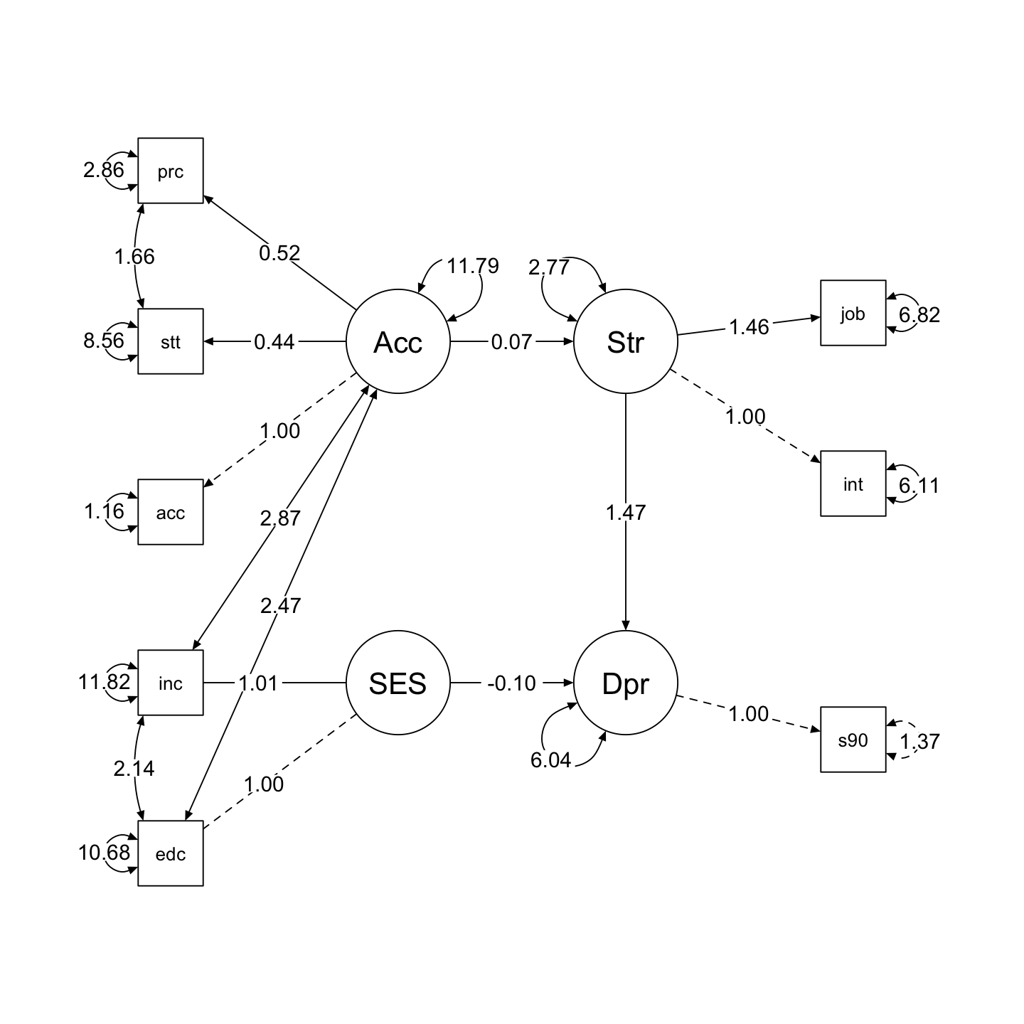
# figure 16.2(c)
lavaan::summary(shenSESnoComposite, header = FALSE, fit.measures = FALSE,
 standardized = TRUE, rsquare = TRUE) |> print()
Parameter Estimates:

  Standard errors                             Standard
  Information                                 Expected
  Information saturated (h1) model          Structured

Latent Variables:
                   Estimate  Std.Err  z-value  P(>|z|)   Std.lv  Std.all
  Acculturation =~
    acculscl          1.000                               3.434    0.954
    status            0.444    0.050    8.784    0.000    1.523    0.462
    percent           0.516    0.051   10.070    0.000    1.771    0.723
  Stress =~
    interpers         1.000                               1.679    0.562
    job               1.456    0.125   11.655    0.000    2.445    0.683
  Depression =~
    scl90d            1.000                               3.502    0.948

Regressions:
                   Estimate  Std.Err  z-value  P(>|z|)   Std.lv  Std.all
  Stress ~
    Acculturation     0.068    0.021    3.241    0.001    0.139    0.139
  Depression ~
    educ             -0.095    0.032   -3.014    0.003   -0.027   -0.089
    income           -0.096    0.030   -3.209    0.001   -0.027   -0.095
    Stress            1.469    0.126   11.704    0.000    0.704    0.704

Covariances:
                   Estimate  Std.Err  z-value  P(>|z|)   Std.lv  Std.all
 .status ~~
   .percent           1.665    0.307    5.424    0.000    1.665    0.336
  Acculturation ~~
    income            2.871    0.404    7.101    0.000    0.836    0.243
    educ              2.469    0.382    6.455    0.000    0.719    0.220
  educ ~~
    income            2.135    0.365    5.852    0.000    2.135    0.190

Variances:
                   Estimate  Std.Err  z-value  P(>|z|)   Std.lv  Std.all
   .scl90d            1.369                               1.369    0.100
   .acculscl          1.157    1.115    1.038    0.299    1.157    0.089
   .status            8.559    0.451   18.997    0.000    8.559    0.787
   .percent           2.862    0.323    8.856    0.000    2.862    0.477
   .interpers         6.112    0.357   17.099    0.000    6.112    0.684
   .job               6.823    0.569   11.988    0.000    6.823    0.533
    educ             10.682    0.482   22.170    0.000   10.682    1.000
    income           11.822    0.533   22.170    0.000   11.822    1.000
    Acculturation    11.790    1.256    9.386    0.000    1.000    1.000
   .Stress            2.765    0.365    7.574    0.000    0.981    0.981
   .Depression        6.036    0.591   10.210    0.000    0.492    0.492

R-Square:
                   Estimate
    scl90d            0.900
    acculscl          0.911
    status            0.213
    percent           0.523
    interpers         0.316
    job               0.467
    Stress            0.019
    Depression        0.508
semPaths2(shenSESnoComposite, layout = "tree", rotation = 2)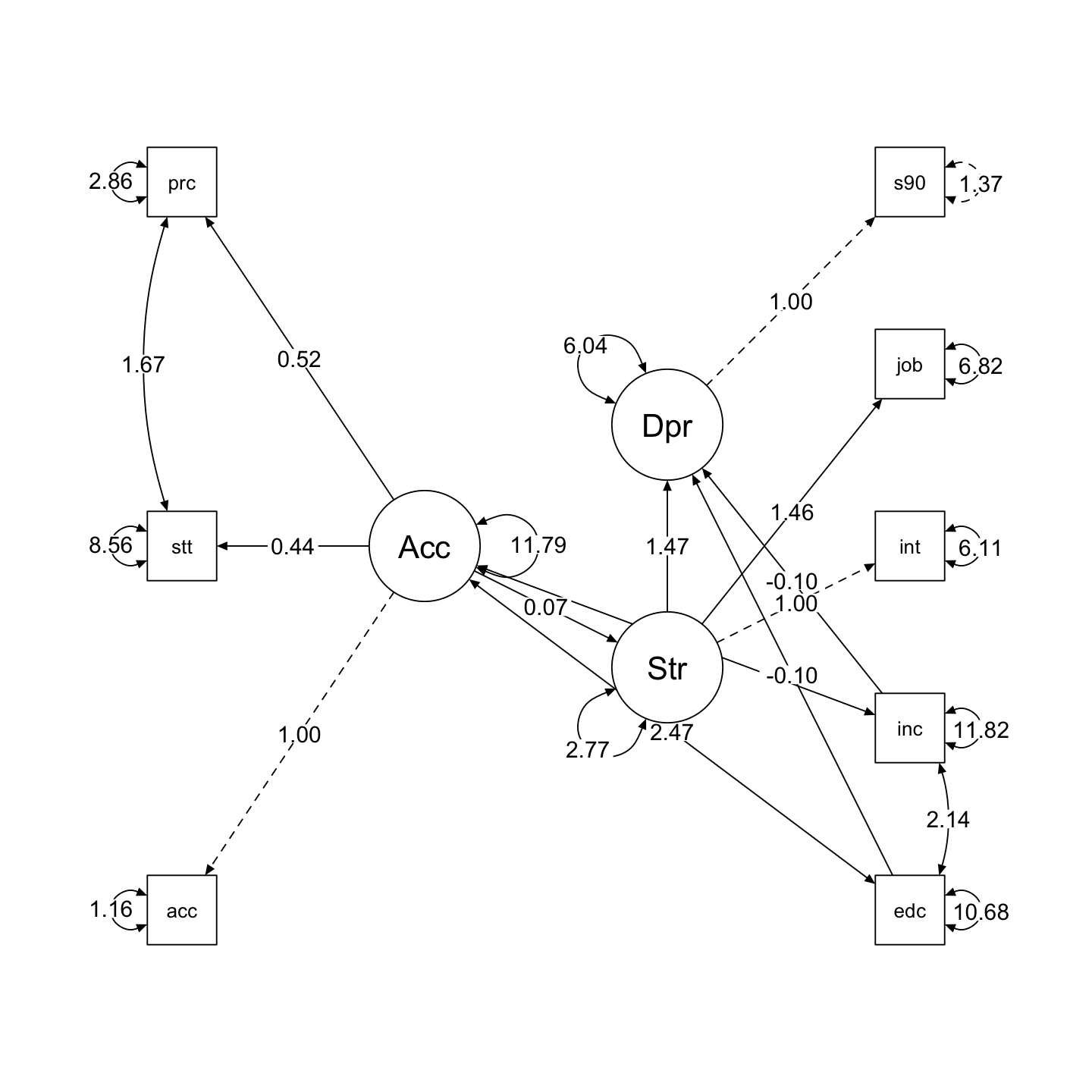
df1 <- parameterEstimates(shenSEScomposite) |>
  mutate(est = est |> round(3)) |>
  select(lhs, op, rhs, est)
df2 <- parameterEstimates(shenSESnoComposite) |>
  mutate(est = est |> round(3)) |>
  select(lhs, op, rhs, est)

# join df1 and df2
full_join(df1, df2, by = c("lhs", "op", "rhs"), suffix = c(".composite", ".noComposite")) |> print()
lhs op rhs est.composite est.noComposite
1 SES <~ educ 1.000 NA
2 SES <~ income 1.013 NA
3 Acculturation =~ acculscl 1.000 1.000
4 Acculturation =~ status 0.444 0.444
5 Acculturation =~ percent 0.516 0.516
6 status ~~ percent 1.665 1.665
7 Stress =~ interpers 1.000 1.000
8 Stress =~ job 1.456 1.456
9 Depression =~ scl90d 1.000 1.000
10 scl90d ~~ scl90d 1.369 1.369
11 Acculturation ~~ income 2.871 2.871
12 Acculturation ~~ educ 2.469 2.469
13 educ ~~ income 2.135 2.135
14 SES ~~ Acculturation 0.000 NA
15 Stress ~ Acculturation 0.068 0.068
16 Depression ~ SES -0.095 NA
17 Depression ~ Stress 1.469 1.469
18 acculscl ~~ acculscl 1.157 1.157
19 status ~~ status 8.559 8.559
20 percent ~~ percent 2.862 2.862
21 interpers ~~ interpers 6.112 6.112
22 job ~~ job 6.823 6.823
23 educ ~~ educ 10.682 10.682
24 income ~~ income 11.822 11.822
25 SES ~~ SES 0.000 NA
26 Acculturation ~~ Acculturation 11.790 11.790
27 Stress ~~ Stress 2.765 2.765
28 Depression ~~ Depression 6.036 6.036
29 Depression ~ educ NA -0.095
30 Depression ~ income NA -0.096