Load libraries
library(haven)
library(psych)
library(tidyverse)
library(lavaan)
library(semTools)
library(manymome)Multiple Regression and Beyond (3e) by Timothy Z. Keith
library(haven)
library(psych)
library(tidyverse)
library(lavaan)
library(semTools)
library(manymome)covariance matrix
공분산 covariance of \(x, ~ y\): \(Cov(x, y)\) = \(\displaystyle\frac{1}{n-1} \sum_{i=1}^{n} (x_i - \bar{x})(y_i - \bar{y})\)
분산 variance of \(x\): covarance of \(x, ~ x\): \(V(x) = Cov(x, x)\) = \(\displaystyle\frac{1}{n-1} \sum_{i=1}^{n} (x_i - \bar{x})^2\)
상관 correlation of \(x, ~ y\): \(Cor(x, y)\) = \(\displaystyle\frac{Cov(x, y)}{\sigma_x \sigma_y}\)
where \(\sigma_x\) and \(\sigma_y\) are the standard deviations of x and y respectively.
변수들 간의 상관계수/공분산 행렬을 알면 회귀계수를 구할 수 있음. 반대로, 회귀계수들을 알면 상관계수/공분산 행렬을 구할 수 있음.
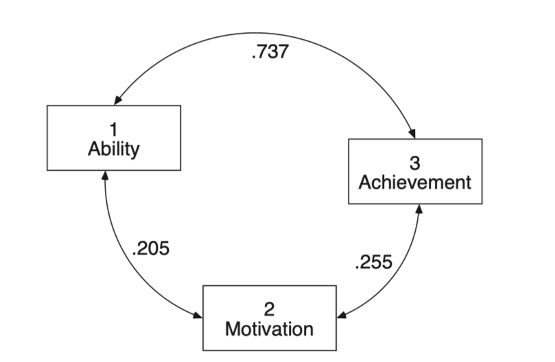
Source: pp. 258-259, Multiple Regression and Beyond (3e) by Timothy Z. Keith
\(a = r_{12}\)
\(\displaystyle b = \frac{r_{13} - r_{12} r_{23}}{1 - r_{12}^2}\)
\(\displaystyle c = \frac{r_{23} - r_{12} r_{13}}{1 - r_{12}^2}\)
# variable names
vars <- c("fam_back", "ability", "motivate", "courses", "achieve")

# Correlation matrix
lower <- "
1.000
.417 1.000
.190 .205 1.000
.372 .498 .375 1.000
.417 .737 .255 .615 1.000"

# standard deviations
sd <- c(1.000, 15.000, 10.000, 2.000, 10.000)

achi_cov <- getCov(lower, names = vars, sd = sd)
achi_cov |> print()
fam_back ability motivate courses achieve
fam_back 1.000 6.255 1.90 0.744 4.17
ability 6.255 225.000 30.75 14.940 110.55
motivate 1.900 30.750 100.00 7.500 25.50
courses 0.744 14.940 7.50 4.000 12.30
achieve 4.170 110.550 25.50 12.300 100.00공분산 행렬을 이용해서 회귀계수를 구하면,
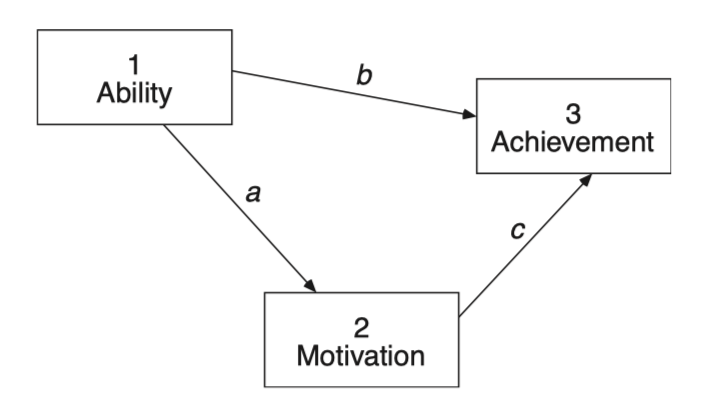
paths <- "
  achieve ~ b*ability + c*motivate
  motivate ~ a*ability
"

achi_model <- sem(paths, sample.cov = achi_cov, sample.nobs = 1000)
parameterEstimates(achi_model, standardized = "std.all", ci = FALSE) |> print()
lhs op rhs label est se z pvalue std.all
1 achieve ~ ability b 0.477 0.014 33.143 0 0.715
2 achieve ~ motivate c 0.108 0.022 5.030 0 0.108
3 motivate ~ ability a 0.137 0.021 6.623 0 0.205
4 achieve ~~ achieve 44.511 1.991 22.361 0 0.446
5 motivate ~~ motivate 95.702 4.280 22.361 0 0.958
6 ability ~~ ability 224.775 0.000 NA NA 1.000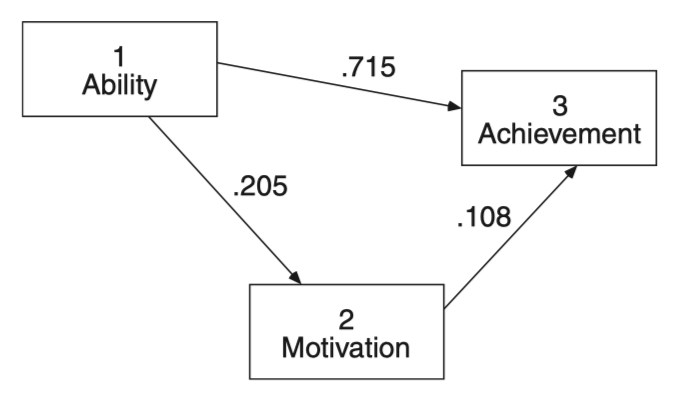
한편, 제한된 다음과 같은 모형에 대한 회귀계수를 구하면,
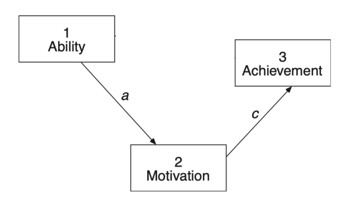
paths <- "
  achieve ~ 0*ability + c*motivate  # ability의 계수를 0으로 고정; 효과 크기 제로!
  motivate ~ a*ability
"

achi_model <- sem(paths, sample.cov = achi_cov, sample.nobs = 100)
parameterEstimates(achi_model, standardized = "std.all", ci = FALSE) |> print()
lhs op rhs label est se z pvalue std.all
1 achieve ~ ability 0.000 0.000 NA NA 0.000
2 achieve ~ motivate c 0.255 0.097 2.637 0.008 0.255
3 motivate ~ ability a 0.137 0.065 2.094 0.036 0.205
4 achieve ~~ achieve 92.563 13.090 7.071 0.000 0.935
5 motivate ~~ motivate 94.840 13.412 7.071 0.000 0.958
6 ability ~~ ability 222.750 0.000 NA NA 1.000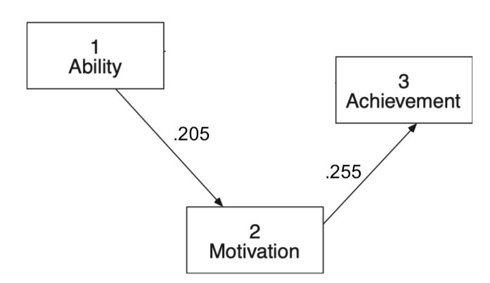
이 때, 이 회귀계수들을 이용해 상관계수를 역으로 계산하면; implied/predicted correlation matrix
# implied/predicted correlation matrix
lavInspect(achi_model, "cor.ov") |>  print()
achiev motivt abilty
achieve 1.000
motivate 0.255 1.000
ability 0.052 0.205 1.000실제 상관계수와 비교해보면,
# observed correlation matrix
achi_cov[c(5, 3, 2), c(5, 3, 2)] |> cov2cor() |> print()
achieve motivate ability
achieve 1.000 0.255 0.737
motivate 0.255 1.000 0.205
ability 0.737 0.205 1.000이 때, 원래의 상관계수를 복구하지 못한다면 데이터와 모형이 맞지 않는다고 볼 수 있음!
lavaan website: estimators and more
기본적으로 ML (Maximum Likelihood) 방법을 사용
# generate a dataset with the same covariance matrix
set.seed(123)
achi <- semTools::kd(achi_cov, n = 1000, type = "exact") |> as_tibble()
achi |> print()
# A tibble: 1,000 x 5
fam_back ability motivate courses achieve
<dbl> <dbl> <dbl> <dbl> <dbl>
1 0.220 -6.13 -2.48 -2.95 -8.33
2 -1.28 -0.980 -6.90 1.99 0.105
3 -1.19 -15.8 -6.33 -1.19 -9.33
4 -1.32 -5.75 2.82 3.14 6.53
5 1.18 12.1 3.58 2.58 3.64
6 1.72 21.7 -9.78 0.0788 11.5
7 -0.629 -4.56 2.07 -2.26 -0.556
8 -0.559 -6.81 -7.23 -0.0846 -3.99
9 0.706 10.4 18.6 2.09 21.5
10 1.02 4.77 11.2 1.17 5.92
# i 990 more rows# check the covariance matrix
cov(achi) |> print() fam_back ability motivate courses achieve
fam_back 1.0010010 6.261261 1.901902 0.7447447 4.174174
ability 6.2612613 225.225225 30.780781 14.9549550 110.660661
motivate 1.9019019 30.780781 100.100100 7.5075075 25.525526
courses 0.7447447 14.954955 7.507508 4.0040040 12.312312
achieve 4.1741742 110.660661 25.525526 12.3123123 100.100100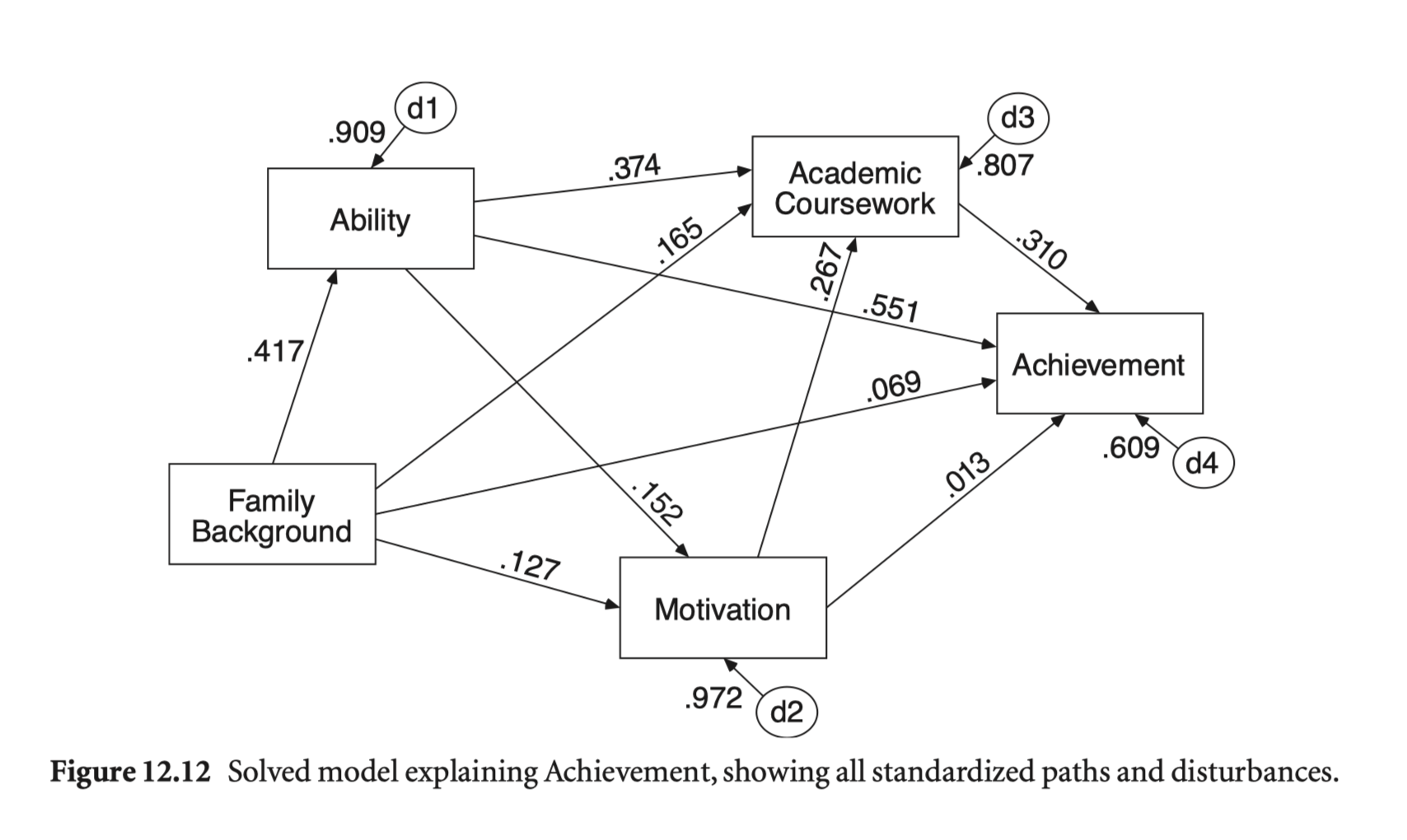
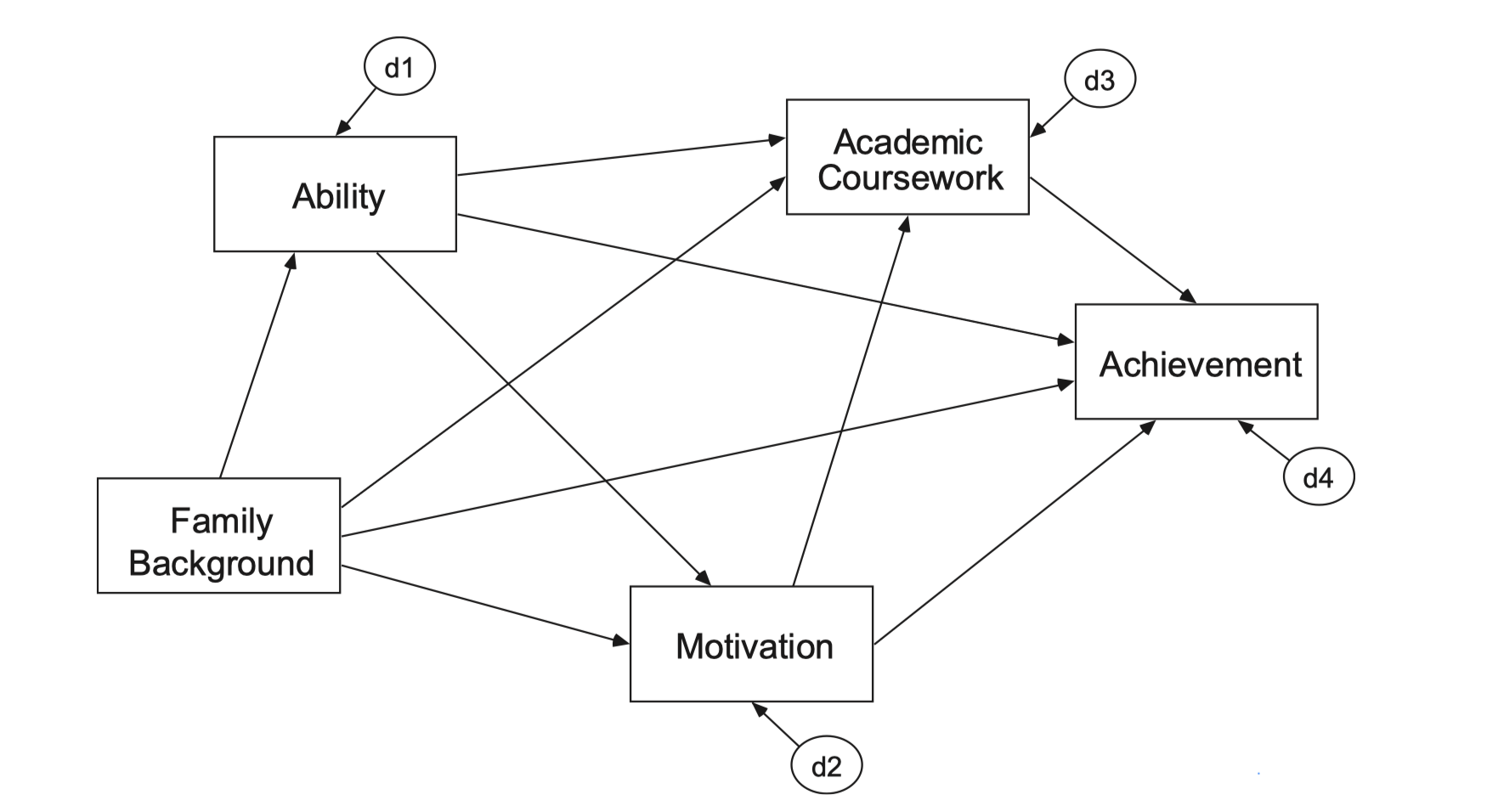
Source: p. 270, Multiple Regression and Beyond (3e) by Timothy Z. Keith
achi_paths <- "
  achieve ~ fam_back + ability + motivate + courses
  courses ~ fam_back + ability + motivate
  motivate ~ fam_back + ability
  ability ~ fam_back
"

achi_model <- sem(achi_paths, data = achi)
summary(achi_model, standardized = TRUE, header = FALSE) |> print()
Parameter Estimates:

  Standard errors                             Standard
  Information                                 Expected
  Information saturated (h1) model          Structured

Regressions:
                   Estimate  Std.Err  z-value  P(>|z|)   Std.lv  Std.all
  achieve ~
    fam_back          0.695    0.217    3.202    0.001    0.695    0.069
    ability           0.367    0.015   23.758    0.000    0.367    0.551
    motivate          0.013    0.021    0.604    0.546    0.013    0.013
    courses           1.550    0.119   12.996    0.000    1.550    0.310
  courses ~
    fam_back          0.330    0.057    5.838    0.000    0.330    0.165
    ability           0.050    0.004   13.194    0.000    0.050    0.374
    motivate          0.053    0.005   10.158    0.000    0.053    0.267
  motivate ~
    fam_back          1.265    0.338    3.741    0.000    1.265    0.127
    ability           0.101    0.023    4.502    0.000    0.101    0.152
  ability ~
    fam_back          6.255    0.431   14.508    0.000    6.255    0.417

Variances:
                   Estimate  Std.Err  z-value  P(>|z|)   Std.lv  Std.all
   .achieve          37.103    1.659   22.361    0.000   37.103    0.371
   .courses           2.608    0.117   22.361    0.000    2.608    0.652
   .motivate         94.475    4.225   22.361    0.000   94.475    0.945
   .ability         185.875    8.313   22.361    0.000  185.875    0.826
1 - 잔차의 표준화된 분산(variance): .xxxx 표시
직접 출력하는 옵션: rsquare = TRUE
summary(achi_model, standardized = TRUE, rsquare = TRUE, header = FALSE) |> print()
Parameter Estimates:

  Standard errors                            Bootstrap
  Number of requested bootstrap draws             1000
  Number of successful bootstrap draws             965

Regressions:
                   Estimate  Std.Err  z-value  P(>|z|)   Std.lv  Std.all
  achieve ~
    fam_back          0.695    0.221    3.141    0.002    0.695    0.069
    ability           0.367    0.016   23.074    0.000    0.367    0.551
    motivate   (a)    0.013    0.021    0.610    0.542    0.013    0.013
    courses   (b1)    1.550    0.119   12.974    0.000    1.550    0.310
  courses ~
    fam_back          0.330    0.059    5.604    0.000    0.330    0.165
    ability           0.050    0.004   13.685    0.000    0.050    0.374
    motivate  (b2)    0.053    0.005    9.984    0.000    0.053    0.267
  motivate ~
    fam_back          1.265    0.331    3.826    0.000    1.265    0.127
    ability           0.101    0.024    4.270    0.000    0.101    0.152
  ability ~
    fam_back          6.255    0.433   14.455    0.000    6.255    0.417

Variances:
                   Estimate  Std.Err  z-value  P(>|z|)   Std.lv  Std.all
   .achieve          37.103    1.730   21.450    0.000   37.103    0.371
   .courses           2.608    0.121   21.579    0.000    2.608    0.652
   .motivate         94.475    4.205   22.470    0.000   94.475    0.945
   .ability         185.875    8.120   22.891    0.000  185.875    0.826

R-Square:
                   Estimate
    achieve           0.629
    courses           0.348
    motivate          0.055
    ability           0.174

Defined Parameters:
                   Estimate  Std.Err  z-value  P(>|z|)   Std.lv  Std.all
    indirect          0.083    0.011    7.739    0.000    0.083    0.083
    total             0.095    0.021    4.549    0.000    0.095    0.095
header: TRUEfit.measures: FALSEestimates: TRUEci: FALSEfmi: FALSEstandardized: FALSE / “std.all”, “std.lv”rsquare: FALSEmodindices: FALSEstd.nox: FALSEremove.step1: TRUEremove.unused: TRUEcov.std: TRUEnd: 3Llavaan doc 참고;
If header = TRUE, the header section (including fit measures) is printed.
If fit.measures = TRUE, additional fit measures are added to the header section. The related fm.args list allows to set options related to the fit measures. See fitMeasures for more details.
If estimates = TRUE, print the parameter estimates section.
If ci = TRUE, add confidence intervals to the parameter estimates section.
If fmi = TRUE, add the fmi (fraction of missing information) column, if it is available.
If standardized=TRUE or a character vector, the standardized solution is also printed (see parameterEstimates). Note that SEs and tests are still based on unstandardized estimates. Use standardizedSolution to obtain SEs and test statistics for standardized estimates.
The std.nox argument is deprecated; the standardized argument allows “std.nox” solution to be specifically requested.
If remove.step1, the parameters of the measurement part are not shown (only used when using sam().) If remove.unused, automatically added parameters that are fixed to their default (0 or 1) values are removed.
If rsquare=TRUE, the R-Square values for the dependent variables in the model are printed.
If efa = TRUE, EFA related information is printed. The related efa.args list allows to set options related to the EFA output. See summary.efaList for more details.
If modindices=TRUE, modification indices are printed for all fixed parameters.
The argument nd determines the number of digits after the decimal point to be printed (currently only in the parameter estimates section.)
Direct, Indirect, and Total Effects
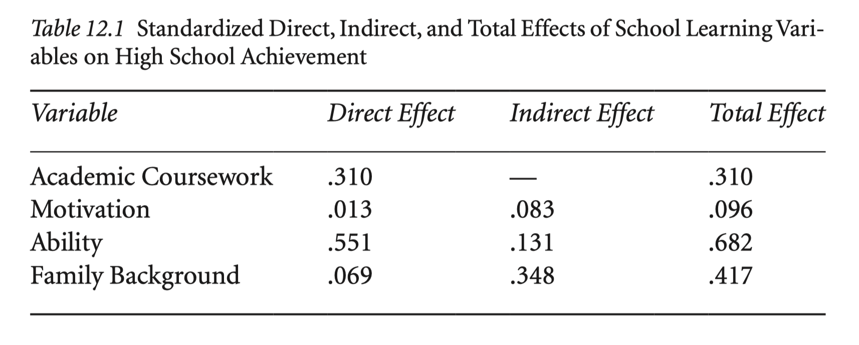
Source: p. 272, Multiple Regression and Beyond (3e) by Timothy Z. Keith
movivation -> achievement
achi_paths <- "
  achieve ~ fam_back + ability + a*motivate + b1*courses
  courses ~ fam_back + ability + b2*motivate
  motivate ~ fam_back + ability
  ability ~ fam_back

  indirect := b1*b2
  total := a + b1*b2
"

achi_model <- sem(achi_paths, data = achi)
summary(achi_model, standardized = TRUE, header = FALSE) |> print()
Parameter Estimates:

  Standard errors                             Standard
  Information                                 Expected
  Information saturated (h1) model          Structured

Regressions:
                   Estimate  Std.Err  z-value  P(>|z|)   Std.lv  Std.all
  achieve ~
    fam_back          0.695    0.217    3.202    0.001    0.695    0.069
    ability           0.367    0.015   23.758    0.000    0.367    0.551
    motivate   (a)    0.013    0.021    0.604    0.546    0.013    0.013
    courses   (b1)    1.550    0.119   12.996    0.000    1.550    0.310
  courses ~
    fam_back          0.330    0.057    5.838    0.000    0.330    0.165
    ability           0.050    0.004   13.194    0.000    0.050    0.374
    motivate  (b2)    0.053    0.005   10.158    0.000    0.053    0.267
  motivate ~
    fam_back          1.265    0.338    3.741    0.000    1.265    0.127
    ability           0.101    0.023    4.502    0.000    0.101    0.152
  ability ~
    fam_back          6.255    0.431   14.508    0.000    6.255    0.417

Variances:
                   Estimate  Std.Err  z-value  P(>|z|)   Std.lv  Std.all
   .achieve          37.103    1.659   22.361    0.000   37.103    0.371
   .courses           2.608    0.117   22.361    0.000    2.608    0.652
   .motivate         94.475    4.225   22.361    0.000   94.475    0.945
   .ability         185.875    8.313   22.361    0.000  185.875    0.826

Defined Parameters:
                   Estimate  Std.Err  z-value  P(>|z|)   Std.lv  Std.all
    indirect          0.083    0.010    8.003    0.000    0.083    0.083
    total             0.095    0.021    4.448    0.000    0.095    0.095
Bootstrapping으로 추정
achi_model <- sem(
  achi_paths,
  data = achi,
  se = "bootstrap",  # standard errors
  bootstrap = 1000,  # number of bootstrap samples
)
summary(achi_model, standardized = TRUE, header = FALSE, ci = TRUE) |> print()
Parameter Estimates:

  Standard errors                            Bootstrap
  Number of requested bootstrap draws             1000
  Number of successful bootstrap draws             962

Regressions:
                   Estimate  Std.Err  z-value  P(>|z|) ci.lower ci.upper
  achieve ~
    fam_back          0.695    0.214    3.253    0.001    0.272    1.150
    ability           0.367    0.016   23.685    0.000    0.334    0.396
    motivate   (a)    0.013    0.020    0.625    0.532   -0.027    0.052
    courses   (b1)    1.550    0.121   12.767    0.000    1.313    1.771
  courses ~
    fam_back          0.330    0.057    5.814    0.000    0.211    0.437
    ability           0.050    0.004   13.570    0.000    0.043    0.057
    motivate  (b2)    0.053    0.005   10.221    0.000    0.043    0.063
  motivate ~
    fam_back          1.265    0.351    3.607    0.000    0.568    1.973
    ability           0.101    0.025    4.112    0.000    0.054    0.147
  ability ~
    fam_back          6.255    0.436   14.350    0.000    5.396    7.099
   Std.lv  Std.all

    0.695    0.069
    0.367    0.551
    0.013    0.013
    1.550    0.310

    0.330    0.165
    0.050    0.374
    0.053    0.267

    1.265    0.127
    0.101    0.152

    6.255    0.417

Variances:
                   Estimate  Std.Err  z-value  P(>|z|) ci.lower ci.upper
   .achieve          37.103    1.718   21.601    0.000   33.508   40.317
   .courses           2.608    0.116   22.453    0.000    2.363    2.842
   .motivate         94.475    4.170   22.656    0.000   85.326  102.484
   .ability         185.875    8.044   23.108    0.000  171.185  202.593
   Std.lv  Std.all
   37.103    0.371
    2.608    0.652
   94.475    0.945
  185.875    0.826

Defined Parameters:
                   Estimate  Std.Err  z-value  P(>|z|) ci.lower ci.upper
    indirect          0.083    0.011    7.870    0.000    0.063    0.104
    total             0.095    0.021    4.617    0.000    0.055    0.138
   Std.lv  Std.all
    0.083    0.083
    0.095    0.095
parameterEstimates(
  achi_model,
  boot.ci.type = "bca.simple", # bias-corrected
  standardized = "std.all" # standardized estimates
) |> filter(label != "") |> print()
lhs op rhs label est se z pvalue ci.lower ci.upper
1 achieve ~ motivate a 0.013 0.020 0.625 0.532 -0.027 0.053
2 achieve ~ courses b1 1.550 0.121 12.767 0.000 1.313 1.771
3 courses ~ motivate b2 0.053 0.005 10.221 0.000 0.044 0.065
4 indirect := b1*b2 indirect 0.083 0.011 7.870 0.000 0.064 0.106
5 total := a+b1*b2 total 0.095 0.021 4.617 0.000 0.057 0.140
std.all
1 0.013
2 0.310
3 0.267
4 0.083
5 0.095패키지를 이용해 경로를 찾아 추정: manymome 참조
library(manymome)

# All specific indirect paths from ability to achieve
paths <- all_indirect_paths(achi_model,
  x = "ability",
  y = "achieve"
)
paths |> print()
Call:
all_indirect_paths(fit = achi_model, x = "ability", y = "achieve")
Path(s):
path
1 ability -> courses -> achieve
2 ability -> motivate -> achieve
3 ability -> motivate -> courses -> achieveind_est_std <- many_indirect_effects(paths,
fit = achi_model, R = 1000,
boot_ci = TRUE, boot_type = "bc",
standardized_x = TRUE,
standardized_y = TRUE
)
ind_est_std
==  Indirect Effect(s) (Both x-variable(s) and y-variable(s) Standardized)  ==
                                            std  CI.lo CI.hi Sig
ability -> courses -> achieve             0.116  0.094 0.140 Sig
ability -> motivate -> achieve            0.002 -0.004 0.010
ability -> motivate -> courses -> achieve 0.013  0.007 0.020 Sig

 - [CI.lo to CI.hi] are 95.0% bias-corrected confidence intervals by
   nonparametric bootstrapping with 1000 samples.
 - std: The standardized indirect effects.
# total indirect effect
ind_est_std[[1]] + ind_est_std[[2]] + ind_est_std[[3]]
== Indirect Effect (Both 'ability' and 'achieve' Standardized) ==

 Path:                ability -> courses -> achieve
 Path:                ability -> motivate -> achieve
 Path:                ability -> motivate -> courses -> achieve
 Function of Effects: 0.131
 95.0% Bootstrap CI:  [0.107 to 0.154]

Computation of the Function of Effects:
 ((ability->courses->achieve)
+(ability->motivate->achieve))
+(ability->motivate->courses->achieve)


Bias-corrected confidence interval formed by nonparametric
bootstrapping with 1000 bootstrap samples.
Total effect = direct effect + total indirect effect
# direct effect
direct_std <- indirect_effect(x = "ability",
                              y = "achieve",
                              fit = achi_model,
                              boot_ci = TRUE, boot_type = "bc",
                              standardized_x = TRUE,
                              standardized_y = TRUE)
direct_std
==  Effect (Both 'ability' and 'achieve' Standardized) ==

 Path:               ability -> achieve
 Effect:             0.551
 95.0% Bootstrap CI: [0.506 to 0.597]

Computation Formula:
  (b.achieve~ability)*sd_ability/sd_achieve
Computation:
  (0.36737)*(15.00000)/(10.00000)

Bias-corrected confidence interval formed by nonparametric
bootstrapping with 1000 bootstrap samples.
direct_std + ind_est_std[[1]] + ind_est_std[[2]] + ind_est_std[[3]]
== Indirect Effect (Both 'ability' and 'achieve' Standardized) ==

 Path:                ability -> achieve
 Path:                ability -> courses -> achieve
 Path:                ability -> motivate -> achieve
 Path:                ability -> motivate -> courses -> achieve
 Function of Effects: 0.682
 95.0% Bootstrap CI:  [0.643 to 0.717]

Computation of the Function of Effects:
 (((ability->achieve)
+(ability->courses->achieve))
+(ability->motivate->achieve))
+(ability->motivate->courses->achieve)


Bias-corrected confidence interval formed by nonparametric
bootstrapping with 1000 bootstrap samples.
위의 모든 간접효과의 합은 중간의 걸친 변수들이 다 제거되었을 때의 효과와 동일
Source: p. 274, Multiple Regression and Beyond (3e) by Timothy Z. Keith
lm(achieve ~ ability + fam_back, data = achi) |> lm.beta::lm.beta() |> print()
Call:
lm(formula = achieve ~ ability + fam_back, data = achi)

Standardized Coefficients::
(Intercept)     ability    fam_back
         NA   0.6816408   0.1327558
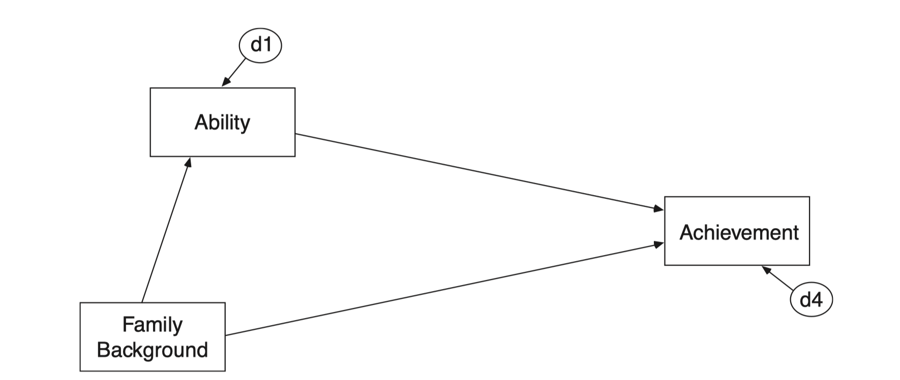
Spurious effect
단순 효과(상관계수) - 총 효과의 크기
lm(achieve ~ ability, data = achi) |> lm.beta::lm.beta() |> print()
Call:
lm(formula = achieve ~ ability, data = achi)

Standardized Coefficients::
(Intercept)     ability
         NA       0.737
achi |> select(achieve, ability) |> lowerCor(digits=3) achiv ablty
achieve 1.000
ability 0.737 1.000# simple effect - total effect
0.737 - 0.681Table 12.1에서 familiy background에 대해서도 동일한 분석을 수행해보세요.
예전 salary 데이터에 대해서도 동일한 분석을 수행해보세요; 링크