Load libraries
library(tidyverse)
library(lavaan)
library(semTools)Multiple Regression and Beyond (3e) by Timothy Z. Keith
library(tidyverse)
library(lavaan)
library(semTools)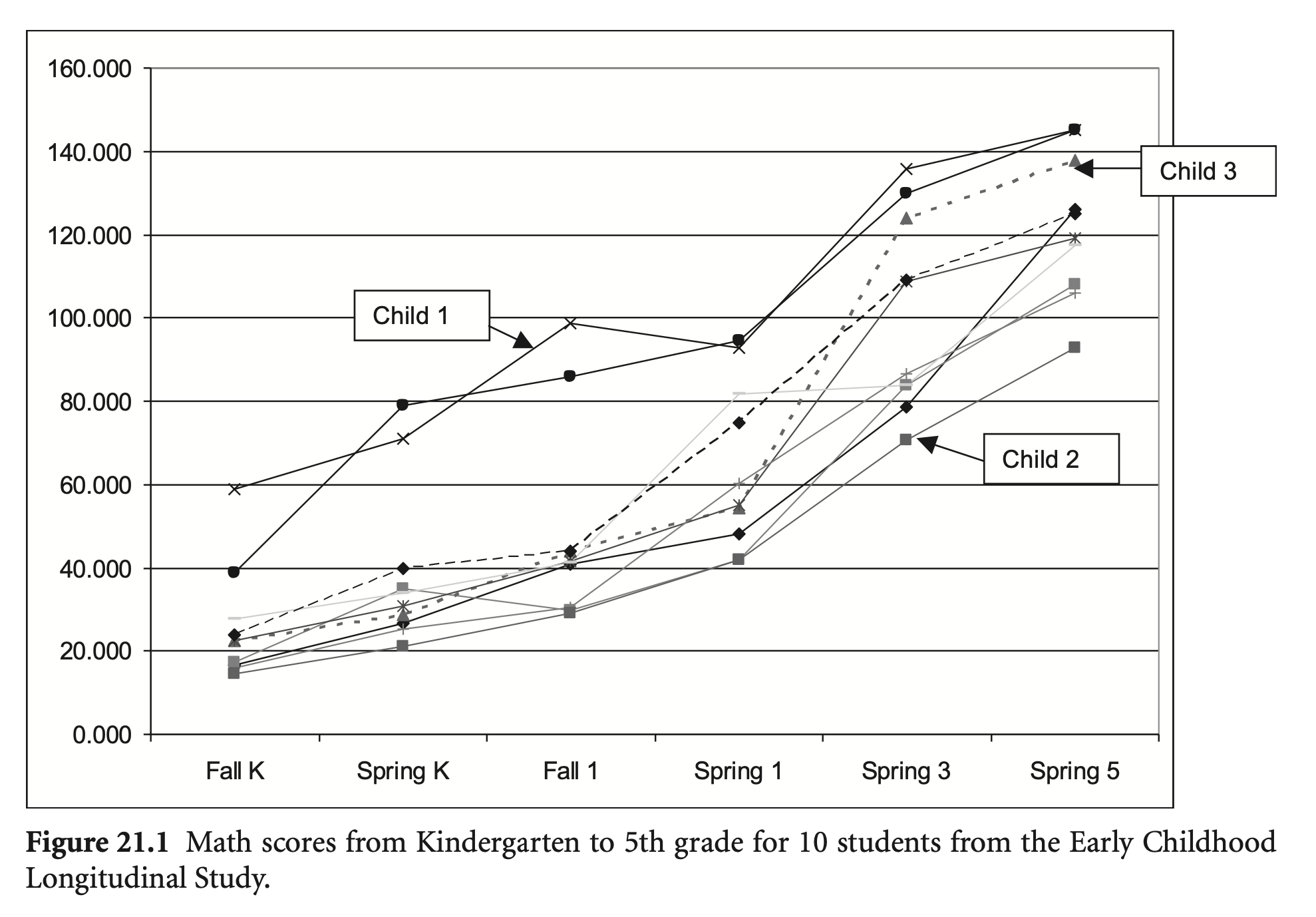
데이터는 다음 연구를 기반으로 생성
DiPerna, J. C., Lei, P. W., & Reid, E. E. (2007). Kindergarten predictors of mathematical growth in the primary grades: An investigation using the Early Childhood Longitudinal Study–Kindergarten cohort. Journal of Educational psychology, 99(2), 369.
math1 ~ math5: 유치원, 1, 2, 3, 4학년까지의 수학 성적
The test is designed to measure “conceptual knowledge, procedural knowledge, and problem solving” with math items ranging from simple (number knowledge) to advanced (algebra) (DiPerna, Lei, & Reid, 2007, p. 372)
math_growth <- haven::read_sav("data/chap 21 latent growth models/math growth final.sav")
math_growth |> print()
# A tibble: 1,000 × 9
math1 math2 math3 math4 math5 sex age ParEd Cognitive
<dbl> <dbl> <dbl> <dbl> <dbl> <dbl> <dbl> <dbl> <dbl>
1 57.4 65.8 78.7 86.0 93.8 1 68.2 16 95
2 81.4 87.9 94.2 104. 111. 1 70.8 15 104
3 74.7 82.0 95.5 109. 120. 0 65.4 15 107
4 71.1 80.4 88.2 97.8 102. 1 68.9 14 121
5 70.1 79.1 85.2 92.1 102. 1 69.8 17 112
6 71.7 84.2 86.2 88.2 94.9 0 67.5 19 69
# ℹ 994 more rows# 분포 확인: 특히 age
results <- MVN::mvn(data = math_growth, univariatePlot = "histogram") # normality histogram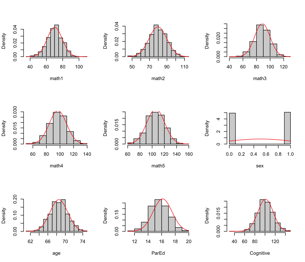
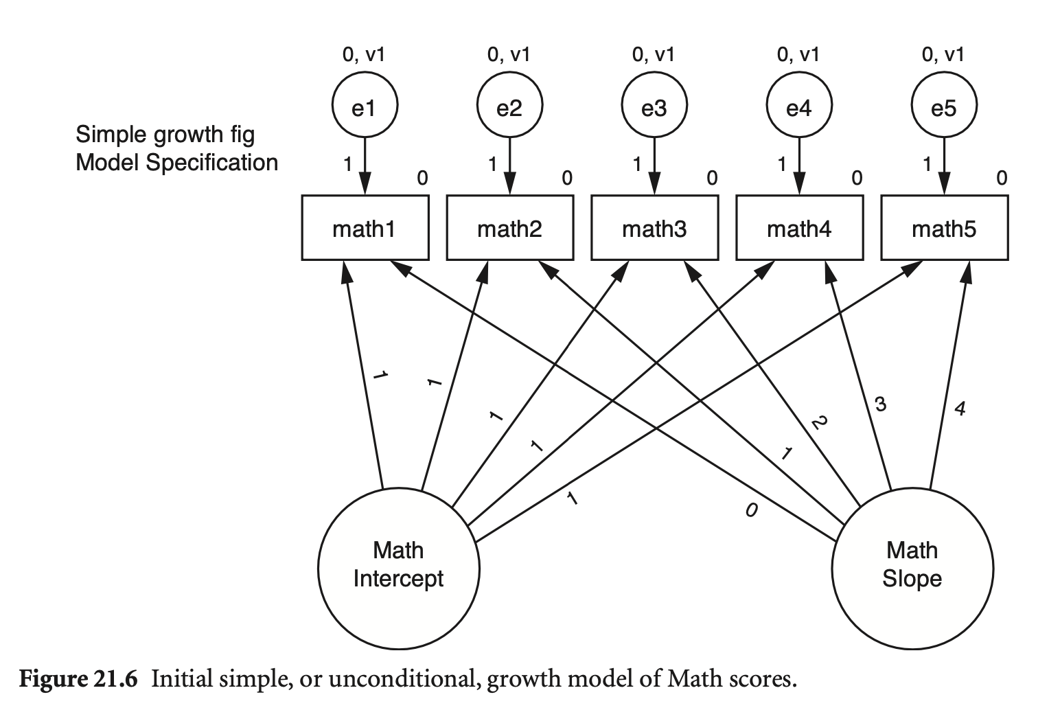
각 indicator들이 두 잠재변수(\(\xi_1, ~\xi_2\))에 의해 예측되는 모형
\(math1 = 0\cdot Slope + 1\cdot Intercept + 0\)
\(math2 = 1\cdot Slope + 1\cdot Intercept + 0\)
\(math3 = 2\cdot Slope + 1\cdot Intercept + 0\)
\(math4 = 3\cdot Slope + 1\cdot Intercept + 0\)
\(math5 = 4\cdot Slope + 1\cdot Intercept + 0\)
\(math = Slope\cdot X + Intercept\cdot 1\), \(X = 0, 1, 2, 3, 4\)
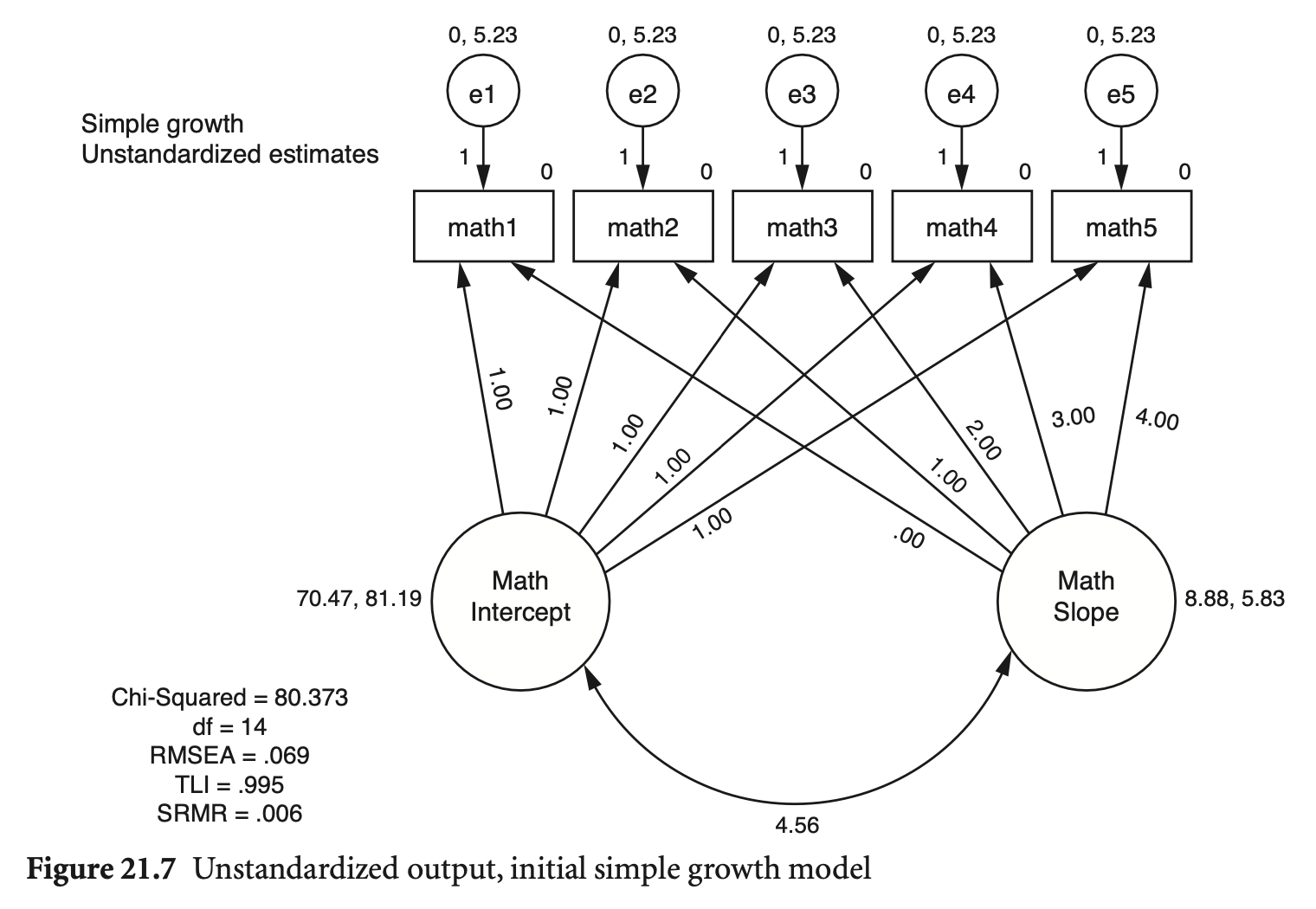
# Unconditional growth model
lgm_math_model <- '
  # latents
  Initial =~ 1*math1 + 1*math2 + 1*math3 + 1*math4 + 1*math5
  Growth =~ 0*math1 + 1*math2 + 2*math3 + 3*math4 + 4*math5

  # intercepts
  Initial ~ 1
  Growth ~ 1

  # residual (co)variances
  Growth ~~ Initial

  math1 ~~ a*math1
  math2 ~~ a*math2
  math3 ~~ a*math3
  math4 ~~ a*math4
  math5 ~~ a*math5

  # not neeed when using growth() function instead sem()
  math1 ~ 0*1
  math2 ~ 0*1
  math3 ~ 0*1
  math4 ~ 0*1
  math5 ~ 0*1
  # same as "math1 + math2 + math3 + math4 + math5 ~ 0*1"
'
lgm_math <- sem(lgm_math_model, data = math_growth)
summary(lgm_math,
        remove.unused = FALSE, # keep the unused parameters
        standardized = TRUE,
        fit.measures = TRUE) |> print()
lavaan 0.6-19 ended normally after 62 iterations
Estimator ML
Optimization method NLMINB
Number of model parameters 10
Number of equality constraints 4
Number of observations 1000
Model Test User Model:
Test statistic 80.454
Degrees of freedom 14
P-value (Chi-square) 0.000
Model Test Baseline Model:
Test statistic 9369.171
Degrees of freedom 10
P-value 0.000
User Model versus Baseline Model:
Comparative Fit Index (CFI) 0.993
Tucker-Lewis Index (TLI) 0.995
Loglikelihood and Information Criteria:
Loglikelihood user model (H0) -14661.484
Loglikelihood unrestricted model (H1) -14621.257
Akaike (AIC) 29334.968
Bayesian (BIC) 29364.414
Sample-size adjusted Bayesian (SABIC) 29345.358
Root Mean Square Error of Approximation:
RMSEA 0.069
90 Percent confidence interval - lower 0.055
90 Percent confidence interval - upper 0.084
P-value H_0: RMSEA <= 0.050 0.015
P-value H_0: RMSEA >= 0.080 0.115
Standardized Root Mean Square Residual:
SRMR 0.017
Parameter Estimates:
Standard errors Standard
Information Expected
Information saturated (h1) model Structured
Latent Variables:
Estimate Std.Err z-value P(>|z|) Std.lv Std.all
Initial =~
math1 1.000 9.010 0.969
math2 1.000 9.010 0.895
math3 1.000 9.010 0.797
math4 1.000 9.010 0.699
math5 1.000 9.010 0.613
Growth =~
math1 0.000 0.000 0.000
math2 1.000 2.414 0.240
math3 2.000 4.828 0.427
math4 3.000 7.241 0.562
math5 4.000 9.655 0.657
Covariances:
Estimate Std.Err z-value P(>|z|) Std.lv Std.all
Initial ~~
Growth 4.559 0.741 6.156 0.000 0.210 0.210
Intercepts:
Estimate Std.Err z-value P(>|z|) Std.lv Std.all
Initial 70.467 0.290 242.668 0.000 7.821 7.821
Growth 8.877 0.080 111.410 0.000 3.678 3.678
.math1 0.000 0.000 0.000
.math2 0.000 0.000 0.000
.math3 0.000 0.000 0.000
.math4 0.000 0.000 0.000
.math5 0.000 0.000 0.000
Variances:
Estimate Std.Err z-value P(>|z|) Std.lv Std.all
.math1 (a) 5.228 0.135 38.730 0.000 5.228 0.060
.math2 (a) 5.228 0.135 38.730 0.000 5.228 0.052
.math3 (a) 5.228 0.135 38.730 0.000 5.228 0.041
.math4 (a) 5.228 0.135 38.730 0.000 5.228 0.031
.math5 (a) 5.228 0.135 38.730 0.000 5.228 0.024
Initial 81.187 3.772 21.524 0.000 1.000 1.000
Growth 5.826 0.284 20.496 0.000 1.000 1.000
sem() 대신 growth()를 이용하면,
# Unconditional growth model
lgm_math_model <- '
  # latents
  Initial =~ 1*math1 + 1*math2 + 1*math3 + 1*math4 + 1*math5
  Growth =~ 0*math1 + 1*math2 + 2*math3 + 3*math4 + 4*math5

  # intercepts
  Initial ~ 1
  Growth ~ 1

  # residual (co)variances
  Growth ~~ Initial

  math1 ~~ a*math1
  math2 ~~ a*math2
  math3 ~~ a*math3
  math4 ~~ a*math4
  math5 ~~ a*math5
'
lgm_math <- growth(lgm_math_model, data = math_growth)
summary(lgm_math,
        remove.unused = FALSE, # keep the unused parameters
        standardized = TRUE,
        fit.measures = TRUE) |> print()
lavaan 0.6-19 ended normally after 62 iterations
Estimator ML
Optimization method NLMINB
Number of model parameters 10
Number of equality constraints 4
Number of observations 1000
Model Test User Model:
Test statistic 80.454
Degrees of freedom 14
P-value (Chi-square) 0.000
Model Test Baseline Model:
Test statistic 9369.171
Degrees of freedom 10
P-value 0.000
User Model versus Baseline Model:
Comparative Fit Index (CFI) 0.993
Tucker-Lewis Index (TLI) 0.995
Loglikelihood and Information Criteria:
Loglikelihood user model (H0) -14661.484
Loglikelihood unrestricted model (H1) -14621.257
Akaike (AIC) 29334.968
Bayesian (BIC) 29364.414
Sample-size adjusted Bayesian (SABIC) 29345.358
Root Mean Square Error of Approximation:
RMSEA 0.069
90 Percent confidence interval - lower 0.055
90 Percent confidence interval - upper 0.084
P-value H_0: RMSEA <= 0.050 0.015
P-value H_0: RMSEA >= 0.080 0.115
Standardized Root Mean Square Residual:
SRMR 0.017
Parameter Estimates:
Standard errors Standard
Information Expected
Information saturated (h1) model Structured
Latent Variables:
Estimate Std.Err z-value P(>|z|) Std.lv Std.all
Initial =~
math1 1.000 9.010 0.969
math2 1.000 9.010 0.895
math3 1.000 9.010 0.797
math4 1.000 9.010 0.699
math5 1.000 9.010 0.613
Growth =~
math1 0.000 0.000 0.000
math2 1.000 2.414 0.240
math3 2.000 4.828 0.427
math4 3.000 7.241 0.562
math5 4.000 9.655 0.657
Covariances:
Estimate Std.Err z-value P(>|z|) Std.lv Std.all
Initial ~~
Growth 4.559 0.741 6.156 0.000 0.210 0.210
Intercepts:
Estimate Std.Err z-value P(>|z|) Std.lv Std.all
Initial 70.467 0.290 242.668 0.000 7.821 7.821
Growth 8.877 0.080 111.410 0.000 3.678 3.678
.math1 0.000 0.000 0.000
.math2 0.000 0.000 0.000
.math3 0.000 0.000 0.000
.math4 0.000 0.000 0.000
.math5 0.000 0.000 0.000
Variances:
Estimate Std.Err z-value P(>|z|) Std.lv Std.all
.math1 (a) 5.228 0.135 38.730 0.000 5.228 0.060
.math2 (a) 5.228 0.135 38.730 0.000 5.228 0.052
.math3 (a) 5.228 0.135 38.730 0.000 5.228 0.041
.math4 (a) 5.228 0.135 38.730 0.000 5.228 0.031
.math5 (a) 5.228 0.135 38.730 0.000 5.228 0.024
Initial 81.187 3.772 21.524 0.000 1.000 1.000
Growth 5.826 0.284 20.496 0.000 1.000 1.000
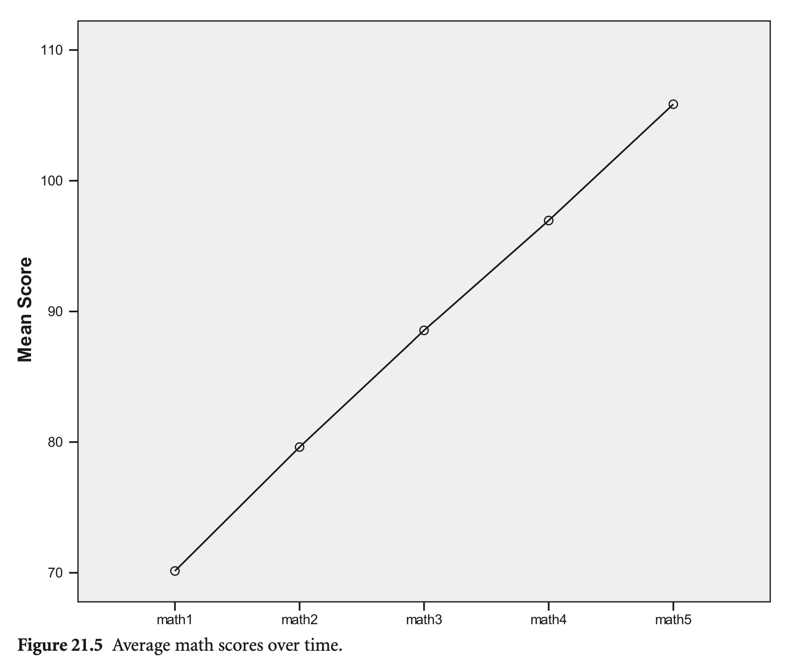
math1, math2, math3, math4, math5에 대해 모형이 예측하는 평균은?
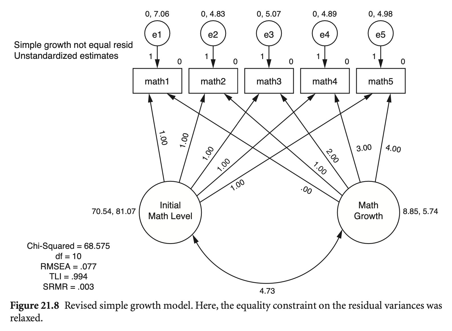
# Unconditional growth model
lgm_math_model_unequal <- '
  # latents
  Initial =~ 1*math1 + 1*math2 + 1*math3 + 1*math4 + 1*math5
  Growth =~ 0*math1 + 1*math2 + 2*math3 + 3*math4 + 4*math5

  # intercepts
  Initial ~ 1
  Growth ~ 1

  # residual (co)variances
  Growth ~~ Initial
'
lgm_math_unequal <- growth(lgm_math_model_unequal, data = math_growth)
summary(lgm_math_unequal,
        remove.unused = FALSE, # keep the unused parameters
        standardized = TRUE,
        fit.measures = TRUE) |> print()
lavaan 0.6-19 ended normally after 160 iterations
Estimator ML
Optimization method NLMINB
Number of model parameters 10
Number of observations 1000
Model Test User Model:
Test statistic 68.644
Degrees of freedom 10
P-value (Chi-square) 0.000
Model Test Baseline Model:
Test statistic 9369.171
Degrees of freedom 10
P-value 0.000
User Model versus Baseline Model:
Comparative Fit Index (CFI) 0.994
Tucker-Lewis Index (TLI) 0.994
Loglikelihood and Information Criteria:
Loglikelihood user model (H0) -14655.579
Loglikelihood unrestricted model (H1) -14621.257
Akaike (AIC) 29331.158
Bayesian (BIC) 29380.235
Sample-size adjusted Bayesian (SABIC) 29348.475
Root Mean Square Error of Approximation:
RMSEA 0.077
90 Percent confidence interval - lower 0.060
90 Percent confidence interval - upper 0.094
P-value H_0: RMSEA <= 0.050 0.005
P-value H_0: RMSEA >= 0.080 0.394
Standardized Root Mean Square Residual:
SRMR 0.018
Parameter Estimates:
Standard errors Standard
Information Expected
Information saturated (h1) model Structured
Latent Variables:
Estimate Std.Err z-value P(>|z|) Std.lv Std.all
Initial =~
math1 1.000 9.004 0.959
math2 1.000 9.004 0.895
math3 1.000 9.004 0.796
math4 1.000 9.004 0.699
math5 1.000 9.004 0.613
Growth =~
math1 0.000 0.000 0.000
math2 1.000 2.395 0.238
math3 2.000 4.790 0.423
math4 3.000 7.185 0.558
math5 4.000 9.580 0.652
Covariances:
Estimate Std.Err z-value P(>|z|) Std.lv Std.all
Initial ~~
Growth 4.729 0.741 6.380 0.000 0.219 0.219
Intercepts:
Estimate Std.Err z-value P(>|z|) Std.lv Std.all
Initial 70.540 0.291 242.420 0.000 7.834 7.834
Growth 8.853 0.079 111.512 0.000 3.696 3.696
.math1 0.000 0.000 0.000
.math2 0.000 0.000 0.000
.math3 0.000 0.000 0.000
.math4 0.000 0.000 0.000
.math5 0.000 0.000 0.000
Variances:
Estimate Std.Err z-value P(>|z|) Std.lv Std.all
.math1 7.064 0.620 11.396 0.000 7.064 0.080
.math2 4.833 0.349 13.845 0.000 4.833 0.048
.math3 5.072 0.289 17.577 0.000 5.072 0.040
.math4 4.889 0.357 13.708 0.000 4.889 0.029
.math5 4.984 0.599 8.313 0.000 4.984 0.023
Initial 81.071 3.790 21.392 0.000 1.000 1.000
Growth 5.736 0.283 20.243 0.000 1.000 1.000
compareFit(lgm_math, lgm_math_unequal) |> summary() |> print()################### Nested Model Comparison #########################
Chi-Squared Difference Test
Df AIC BIC Chisq Chisq diff RMSEA Df diff Pr(>Chisq)
lgm_math_unequal 10 29331 29380 68.644
lgm_math 14 29335 29364 80.454 11.81 0.044187 4 0.01882 *
---
Signif. codes: 0 ‘***’ 0.001 ‘**’ 0.01 ‘*’ 0.05 ‘.’ 0.1 ‘ ’ 1
####################### Model Fit Indices ###########################
chisq df pvalue rmsea cfi tli srmr aic bic
lgm_math_unequal 68.644† 10 .000 .077 .994† .994 .018 29331.158† 29380.235
lgm_math 80.454 14 .000 .069† .993 .995† .017† 29334.968 29364.414†
################## Differences in Fit Indices #######################
df rmsea cfi tli srmr aic bic
lgm_math - lgm_math_unequal 4 -0.008 -0.001 0.001 -0.002 3.81 -15.821
The following lavaan models were compared:
lgm_math_unequal
lgm_math
To view results, assign the compareFit() output to an object and use the summary() method; see the class?FitDiff help page.Unstandardized Estimates
 Standardized Estimates
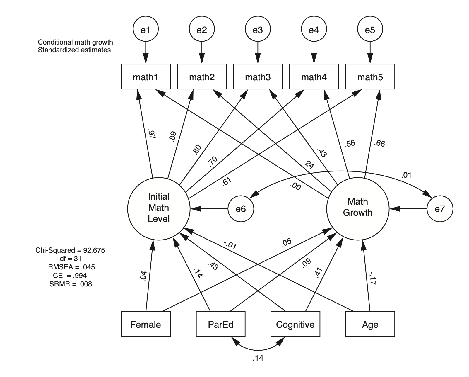
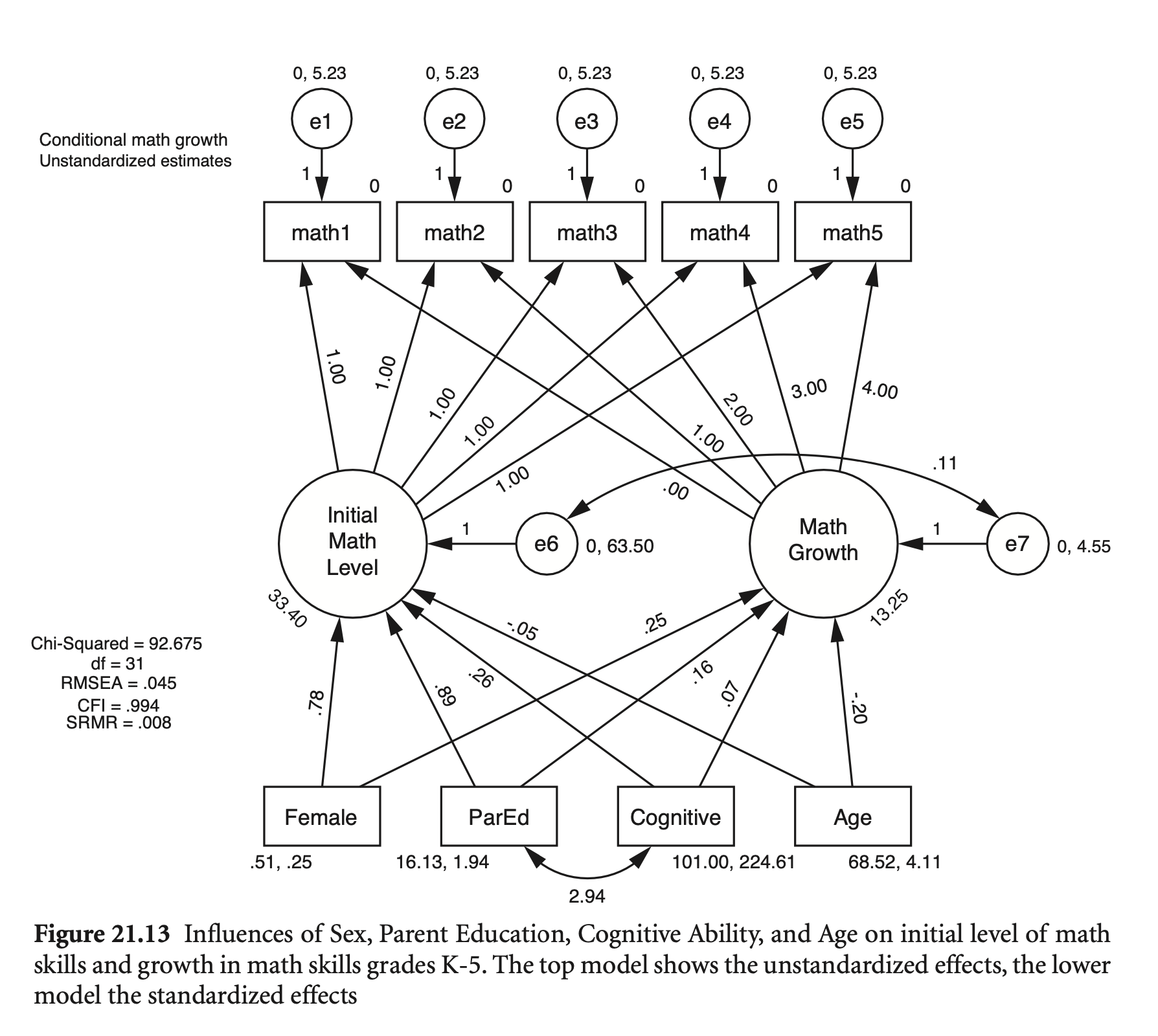
두드러진 점들
# Conditional growth model
lgm_math_cond_model <- '
  # latents
  Initial =~ 1*math1 + 1*math2 + 1*math3 + 1*math4 + 1*math5
  Growth =~ 0*math1 + 1*math2 + 2*math3 + 3*math4 + 4*math5

  # intercepts
  Initial + Growth ~ 1
  sex + ParEd + Cognitive + age ~ 1

  # an alterative syntax for the intercepts
  # Initial ~ 1
  # Growth ~ 1
  # sex ~ 1
  # ParEd ~ 1
  # Cognitive ~ 1
  # age ~ 1

  # residual (co)variances
  Growth ~~ Initial
  ParEd ~~ Cognitive

  math1 ~~ a*math1
  math2 ~~ a*math2
  math3 ~~ a*math3
  math4 ~~ a*math4
  math5 ~~ a*math5

  # regression
  Initial ~ sex +  ParEd + Cognitive + age
  Growth ~ sex + ParEd + Cognitive + age
'
lgm_math_cond <- growth(lgm_math_cond_model, data = math_growth)
summary(lgm_math_cond,
        remove.unused = FALSE, # keep the unused parameters
        standardized = TRUE,
        fit.measures = TRUE) |> print()
lavaan 0.6-19 ended normally after 138 iterations
Estimator ML
Optimization method NLMINB
Number of model parameters 27
Number of equality constraints 4
Number of observations 1000
Model Test User Model:
Test statistic 92.768
Degrees of freedom 31
P-value (Chi-square) 0.000
Model Test Baseline Model:
Test statistic 9839.753
Degrees of freedom 36
P-value 0.000
User Model versus Baseline Model:
Comparative Fit Index (CFI) 0.994
Tucker-Lewis Index (TLI) 0.993
Loglikelihood and Information Criteria:
Loglikelihood user model (H0) -23160.430
Loglikelihood unrestricted model (H1) -23114.046
Akaike (AIC) 46366.859
Bayesian (BIC) 46479.738
Sample-size adjusted Bayesian (SABIC) 46406.688
Root Mean Square Error of Approximation:
RMSEA 0.045
90 Percent confidence interval - lower 0.034
90 Percent confidence interval - upper 0.055
P-value H_0: RMSEA <= 0.050 0.788
P-value H_0: RMSEA >= 0.080 0.000
Standardized Root Mean Square Residual:
SRMR 0.012
Parameter Estimates:
Standard errors Standard
Information Expected
Information saturated (h1) model Structured
Latent Variables:
Estimate Std.Err z-value P(>|z|) Std.lv Std.all
Initial =~
math1 1.000 9.013 0.969
math2 1.000 9.013 0.895
math3 1.000 9.013 0.796
math4 1.000 9.013 0.698
math5 1.000 9.013 0.612
Growth =~
math1 0.000 0.000 0.000
math2 1.000 2.418 0.240
math3 2.000 4.835 0.427
math4 3.000 7.253 0.562
math5 4.000 9.671 0.657
Regressions:
Estimate Std.Err z-value P(>|z|) Std.lv Std.all
Initial ~
sex 0.777 0.516 1.505 0.132 0.086 0.043
ParEd 0.887 0.187 4.738 0.000 0.098 0.137
Cognitive 0.256 0.017 14.709 0.000 0.028 0.426
age -0.051 0.127 -0.400 0.689 -0.006 -0.011
Growth ~
sex 0.246 0.143 1.723 0.085 0.102 0.051
ParEd 0.160 0.052 3.097 0.002 0.066 0.092
Cognitive 0.067 0.005 13.871 0.000 0.028 0.413
age -0.201 0.035 -5.736 0.000 -0.083 -0.169
Covariances:
Estimate Std.Err z-value P(>|z|) Std.lv Std.all
.Initial ~~
.Growth 0.112 0.583 0.192 0.847 0.007 0.007
ParEd ~~
Cognitive 2.940 0.667 4.411 0.000 2.940 0.141
Intercepts:
Estimate Std.Err z-value P(>|z|) Std.lv Std.all
.Initial 33.402 9.322 3.583 0.000 3.706 3.706
.Growth 13.249 2.573 5.149 0.000 5.480 5.480
sex 0.507 0.016 32.069 0.000 0.507 1.014
ParEd 16.133 0.044 366.346 0.000 16.133 11.585
Cognitive 101.001 0.474 213.113 0.000 101.001 6.739
age 68.518 0.064 1068.229 0.000 68.518 33.780
.math1 0.000 0.000 0.000
.math2 0.000 0.000 0.000
.math3 0.000 0.000 0.000
.math4 0.000 0.000 0.000
.math5 0.000 0.000 0.000
Variances:
Estimate Std.Err z-value P(>|z|) Std.lv Std.all
.math1 (a) 5.228 0.135 38.730 0.000 5.228 0.060
.math2 (a) 5.228 0.135 38.730 0.000 5.228 0.052
.math3 (a) 5.228 0.135 38.730 0.000 5.228 0.041
.math4 (a) 5.228 0.135 38.730 0.000 5.228 0.031
.math5 (a) 5.228 0.135 38.730 0.000 5.228 0.024
sex 0.250 0.011 22.361 0.000 0.250 1.000
ParEd 1.939 0.087 22.361 0.000 1.939 1.000
Cognitive 224.611 10.045 22.361 0.000 224.611 1.000
age 4.114 0.184 22.361 0.000 4.114 1.000
.Initial 63.501 2.981 21.300 0.000 0.782 0.782
.Growth 4.554 0.227 20.023 0.000 0.779 0.779
# Conditional growth model - revised
lgm_math_cond_model2 <- '
  # latents
  Initial =~ 1*math1 + 1*math2 + 1*math3 + 1*math4 + 1*math5
  Growth =~ 0*math1 + 1*math2 + 2*math3 + math4 + math5

  # intercepts
  Initial + Growth ~ 1
  sex + ParEd + Cognitive + age ~ 1

  # residual (co)variances
  Growth ~~ 0*Initial # removed covariance
  ParEd ~~ Cognitive

  math1 ~~ a*math1
  math2 ~~ a*math2
  math3 ~~ a*math3
  math4 ~~ a*math4
  math5 ~~ a*math5

  # regression
  Initial ~ ParEd + Cognitive  # remove sex, age
  Growth ~ ParEd + Cognitive + age  # remove sex
'
lgm_math_cond2 <- growth(lgm_math_cond_model2, data = math_growth)
summary(lgm_math_cond2,
        remove.unused = FALSE, # keep the unused parameters
        standardized = TRUE,
        fit.measures = TRUE) |> print()
lavaan 0.6-19 ended normally after 127 iterations
Estimator ML
Optimization method NLMINB
Number of model parameters 25
Number of equality constraints 4
Number of observations 1000
Model Test User Model:
Test statistic 43.024
Degrees of freedom 33
P-value (Chi-square) 0.114
Model Test Baseline Model:
Test statistic 9839.753
Degrees of freedom 36
P-value 0.000
User Model versus Baseline Model:
Comparative Fit Index (CFI) 0.999
Tucker-Lewis Index (TLI) 0.999
Loglikelihood and Information Criteria:
Loglikelihood user model (H0) -23135.558
Loglikelihood unrestricted model (H1) -23114.046
Akaike (AIC) 46313.115
Bayesian (BIC) 46416.178
Sample-size adjusted Bayesian (SABIC) 46349.481
Root Mean Square Error of Approximation:
RMSEA 0.017
90 Percent confidence interval - lower 0.000
90 Percent confidence interval - upper 0.031
P-value H_0: RMSEA <= 0.050 1.000
P-value H_0: RMSEA >= 0.080 0.000
Standardized Root Mean Square Residual:
SRMR 0.017
Parameter Estimates:
Standard errors Standard
Information Expected
Information saturated (h1) model Structured
Latent Variables:
Estimate Std.Err z-value P(>|z|) Std.lv Std.all
Initial =~
math1 1.000 9.001 0.970
math2 1.000 9.001 0.894
math3 1.000 9.001 0.791
math4 1.000 9.001 0.700
math5 1.000 9.001 0.613
Growth =~
math1 0.000 0.000 0.000
math2 1.000 2.507 0.249
math3 2.000 5.015 0.441
math4 2.905 0.013 217.475 0.000 7.284 0.566
math5 3.871 0.018 220.189 0.000 9.706 0.661
Regressions:
Estimate Std.Err z-value P(>|z|) Std.lv Std.all
Initial ~
ParEd 0.883 0.188 4.710 0.000 0.098 0.137
Cognitive 0.254 0.017 14.564 0.000 0.028 0.423
Growth ~
ParEd 0.166 0.054 3.088 0.002 0.066 0.092
Cognitive 0.069 0.005 13.800 0.000 0.027 0.412
age -0.208 0.036 -5.701 0.000 -0.083 -0.168
Covariances:
Estimate Std.Err z-value P(>|z|) Std.lv Std.all
.Initial ~~
.Growth 0.000 0.000 0.000
ParEd ~~
Cognitive 2.940 0.667 4.411 0.000 2.940 0.141
Intercepts:
Estimate Std.Err z-value P(>|z|) Std.lv Std.all
.Initial 30.346 3.289 9.226 0.000 3.371 3.371
.Growth 13.795 2.667 5.172 0.000 5.502 5.502
sex 0.507 0.016 32.069 0.000 0.507 1.014
ParEd 16.133 0.044 366.346 0.000 16.133 11.585
Cognitive 101.001 0.474 213.113 0.000 101.001 6.739
age 68.518 0.064 1068.229 0.000 68.518 33.780
.math1 0.000 0.000 0.000
.math2 0.000 0.000 0.000
.math3 0.000 0.000 0.000
.math4 0.000 0.000 0.000
.math5 0.000 0.000 0.000
Variances:
Estimate Std.Err z-value P(>|z|) Std.lv Std.all
.math1 (a) 5.131 0.132 38.771 0.000 5.131 0.060
.math2 (a) 5.131 0.132 38.771 0.000 5.131 0.051
.math3 (a) 5.131 0.132 38.771 0.000 5.131 0.040
.math4 (a) 5.131 0.132 38.771 0.000 5.131 0.031
.math5 (a) 5.131 0.132 38.771 0.000 5.131 0.024
ParEd 1.939 0.087 22.361 0.000 1.939 1.000
Cognitive 224.611 10.045 22.361 0.000 224.611 1.000
age 4.114 0.184 22.361 0.000 4.114 1.000
sex 0.250 0.011 22.361 0.000 0.250 1.000
.Initial 63.715 2.981 21.374 0.000 0.786 0.786
.Growth 4.921 0.249 19.797 0.000 0.783 0.783
# Compare the two models
compareFit(lgm_math_cond, lgm_math_cond2, nested = FALSE) |> summary() |> print()
####################### Model Fit Indices ###########################
chisq df pvalue rmsea cfi tli srmr aic bic
lgm_math_cond 92.768 31 .000 .045 .994 .993 .012† 46366.859 46479.738
lgm_math_cond2 43.024† 33 .114 .017† 0.999† 0.999† .017 46313.115† 46416.178†
The following lavaan models were compared:
lgm_math_cond
lgm_math_cond2
To view results, assign the compareFit() output to an object and use the summary() method; see the class?FitDiff help page.# Conditional growth model - free slopes
lgm_math_cond_model3 <- '
# latents
Initial =~ 1*math1 + 1*math2 + 1*math3 + 1*math4 + 1*math5
Growth =~ 0*math1 + 1*math2 + 2*math3 + NA*math4 + NA*math5 # free slopes of math4 and math5
# intercepts
Initial + Growth ~ 1
sex + ParEd + Cognitive + age ~ 1
# residual (co)variances
Growth ~~ 0*Initial # removed covariance
ParEd ~~ Cognitive
math1 ~~ a*math1
math2 ~~ a*math2
math3 ~~ a*math3
math4 ~~ a*math4
math5 ~~ a*math5
# regression
Initial ~ ParEd + Cognitive # remove sex, age
Growth ~ ParEd + Cognitive + age # remove sex
'
lgm_math_cond3 <- growth(lgm_math_cond_model3, data = math_growth)
summary(lgm_math_cond3,
remove.unused = FALSE, # keep the unused parameters
standardized = TRUE,
fit.measures = TRUE) |> print()lavaan 0.6-19 ended normally after 127 iterations
Estimator ML
Optimization method NLMINB
Number of model parameters 25
Number of equality constraints 4
Number of observations 1000
Model Test User Model:
Test statistic 43.024
Degrees of freedom 33
P-value (Chi-square) 0.114
Model Test Baseline Model:
Test statistic 9839.753
Degrees of freedom 36
P-value 0.000
User Model versus Baseline Model:
Comparative Fit Index (CFI) 0.999
Tucker-Lewis Index (TLI) 0.999
Loglikelihood and Information Criteria:
Loglikelihood user model (H0) -23135.558
Loglikelihood unrestricted model (H1) -23114.046
Akaike (AIC) 46313.115
Bayesian (BIC) 46416.178
Sample-size adjusted Bayesian (SABIC) 46349.481
Root Mean Square Error of Approximation:
RMSEA 0.017
90 Percent confidence interval - lower 0.000
90 Percent confidence interval - upper 0.031
P-value H_0: RMSEA <= 0.050 1.000
P-value H_0: RMSEA >= 0.080 0.000
Standardized Root Mean Square Residual:
SRMR 0.017
Parameter Estimates:
Standard errors Standard
Information Expected
Information saturated (h1) model Structured
Latent Variables:
Estimate Std.Err z-value P(>|z|) Std.lv Std.all
Initial =~
math1 1.000 9.001 0.970
math2 1.000 9.001 0.894
math3 1.000 9.001 0.791
math4 1.000 9.001 0.700
math5 1.000 9.001 0.613
Growth =~
math1 0.000 0.000 0.000
math2 1.000 2.507 0.249
math3 2.000 5.015 0.441
math4 2.905 0.013 217.475 0.000 7.284 0.566
math5 3.871 0.018 220.189 0.000 9.706 0.661
Regressions:
Estimate Std.Err z-value P(>|z|) Std.lv Std.all
Initial ~
ParEd 0.883 0.188 4.710 0.000 0.098 0.137
Cognitive 0.254 0.017 14.564 0.000 0.028 0.423
Growth ~
ParEd 0.166 0.054 3.088 0.002 0.066 0.092
Cognitive 0.069 0.005 13.800 0.000 0.027 0.412
age -0.208 0.036 -5.701 0.000 -0.083 -0.168
Covariances:
Estimate Std.Err z-value P(>|z|) Std.lv Std.all
.Initial ~~
.Growth 0.000 0.000 0.000
ParEd ~~
Cognitive 2.940 0.667 4.411 0.000 2.940 0.141
Intercepts:
Estimate Std.Err z-value P(>|z|) Std.lv Std.all
.Initial 30.346 3.289 9.226 0.000 3.371 3.371
.Growth 13.795 2.667 5.172 0.000 5.502 5.502
sex 0.507 0.016 32.069 0.000 0.507 1.014
ParEd 16.133 0.044 366.346 0.000 16.133 11.585
Cognitive 101.001 0.474 213.113 0.000 101.001 6.739
age 68.518 0.064 1068.229 0.000 68.518 33.780
.math1 0.000 0.000 0.000
.math2 0.000 0.000 0.000
.math3 0.000 0.000 0.000
.math4 0.000 0.000 0.000
.math5 0.000 0.000 0.000
Variances:
Estimate Std.Err z-value P(>|z|) Std.lv Std.all
.math1 (a) 5.131 0.132 38.771 0.000 5.131 0.060
.math2 (a) 5.131 0.132 38.771 0.000 5.131 0.051
.math3 (a) 5.131 0.132 38.771 0.000 5.131 0.040
.math4 (a) 5.131 0.132 38.771 0.000 5.131 0.031
.math5 (a) 5.131 0.132 38.771 0.000 5.131 0.024
ParEd 1.939 0.087 22.361 0.000 1.939 1.000
Cognitive 224.611 10.045 22.361 0.000 224.611 1.000
age 4.114 0.184 22.361 0.000 4.114 1.000
sex 0.250 0.011 22.361 0.000 0.250 1.000
.Initial 63.715 2.981 21.374 0.000 0.786 0.786
.Growth 4.921 0.249 19.797 0.000 0.783 0.783
# Compare the two models
compareFit(lgm_math_cond, lgm_math_cond3, nested = FALSE) |> summary() |> print()
####################### Model Fit Indices ###########################
chisq df pvalue rmsea cfi tli srmr aic bic
lgm_math_cond 92.768 31 .000 .045 .994 .993 .012† 46366.859 46479.738
lgm_math_cond3 43.024† 33 .114 .017† 0.999† 0.999† .017 46313.115† 46416.178†
The following lavaan models were compared:
lgm_math_cond
lgm_math_cond3
To view results, assign the compareFit() output to an object and use the summary() method; see the class?FitDiff help page.