Load libraries
library(haven)
library(psych)
library(tidyverse)
library(lavaan)
library(semTools)
library(manymome)Multiple Regression and Beyond (3e) by Timothy Z. Keith
library(haven)
library(psych)
library(tidyverse)
library(lavaan)
library(semTools)
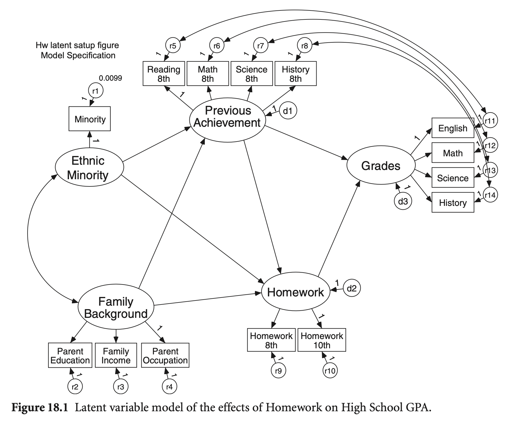
library(manymome)A Latent Variable Homework Model
Single indicators와 correlated errors를 가지는 모형을 구성
hw <- haven::read_sav("data/chap 18 latent var SEM 2/HW latent matrix.sav")
hwcov <- hw[c(2:15), c(3:16)] |>
as.matrix() |>
lav_matrix_vechr(diagonal = TRUE) |>
getCov(names = hw$varname_[2:15], sds = hw[16, 3:16] |> as.double())
# generate a dataset with the same covariance matrix
set.seed(123)
hw_sim <- semTools::kd(hwcov, n = 1000, type = "exact")
# replace Minority values to 1 if it > 0.3, otherwise 0
hw_sim <- hw_sim |>
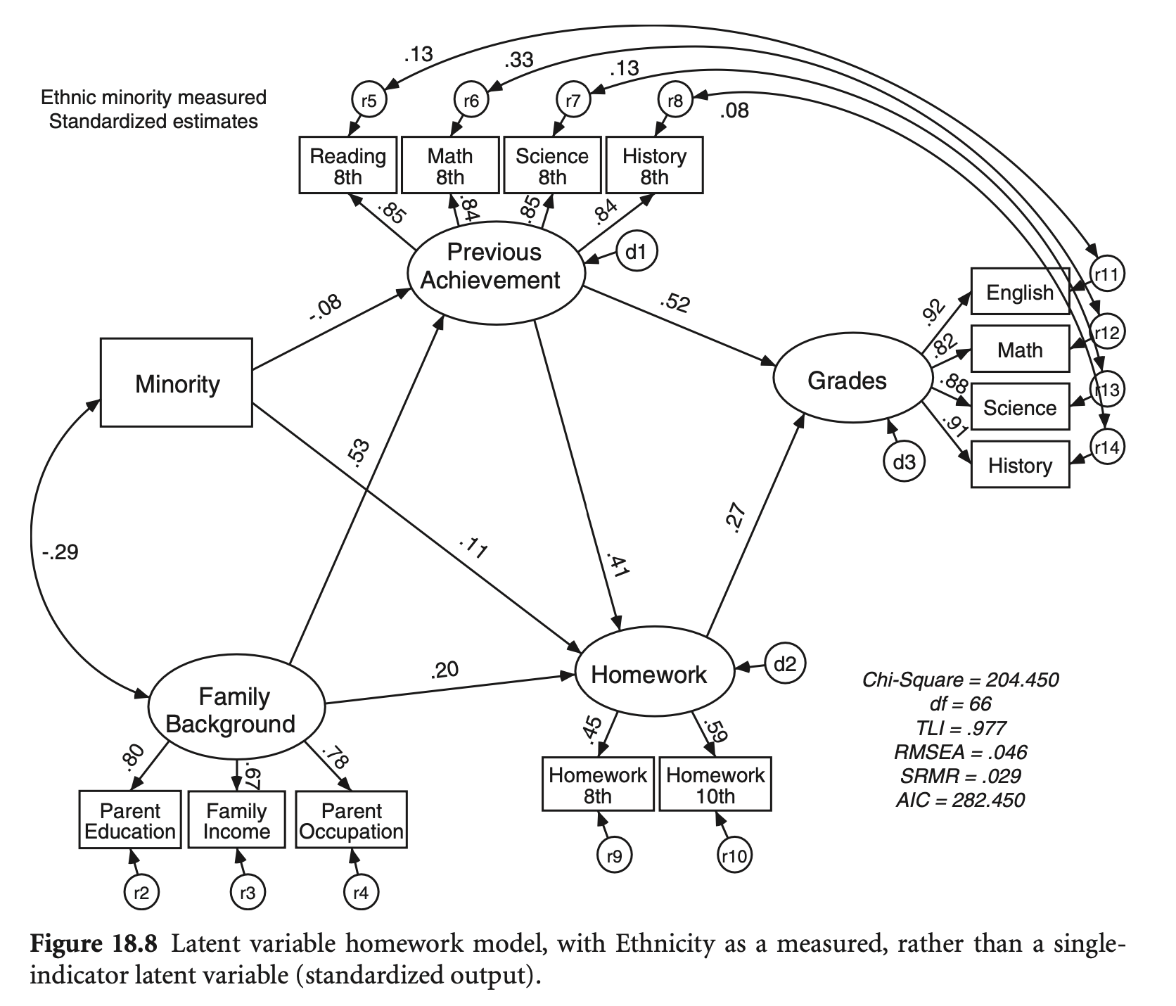
mutate(Minority = ifelse(Minority > 0.3, 1, 0))hw_model <- "
# measurement model
EthnicMinor =~ Minority
Famback =~ parocc + bypared + byfaminc
PrevAch =~ bytxrstd + bytxmstd + bytxsstd + bytxhstd
HW =~ hw10 + hw_8
Grades =~ eng_12 + math_12 + sci_12 + ss_12
# residual covariacne/variance
Minority ~~ 0.0099*Minority
bytxrstd ~~ eng_12
bytxmstd ~~ math_12
bytxsstd ~~ sci_12
bytxhstd ~~ ss_12
# structural model
PrevAch ~ b1*Famback + b2*EthnicMinor
Grades ~ b3*PrevAch + b4*HW
HW ~ b5*PrevAch + b6*Famback + b7*EthnicMinor
# indirect effects; famback > homework > grades
ind_fam := b4*b6
# indirect effects; ethnicminor > homework > grades
ind_ethinic := b4*b7
"
hw_fit <- sem(hw_model, sample.cov = hwcov, sample.nobs = 1000)
summary(hw_fit, standardized = TRUE, fit.measures = TRUE) |> print()lavaan 0.6-19 ended normally after 277 iterations
Estimator ML
Optimization method NLMINB
Number of model parameters 39
Number of observations 1000
Model Test User Model:
Test statistic 204.654
Degrees of freedom 66
P-value (Chi-square) 0.000
Model Test Baseline Model:
Test statistic 8392.044
Degrees of freedom 91
P-value 0.000
User Model versus Baseline Model:
Comparative Fit Index (CFI) 0.983
Tucker-Lewis Index (TLI) 0.977
Loglikelihood and Information Criteria:
Loglikelihood user model (H0) -33331.251
Loglikelihood unrestricted model (H1) -33228.924
Akaike (AIC) 66740.502
Bayesian (BIC) 66931.905
Sample-size adjusted Bayesian (SABIC) 66808.039
Root Mean Square Error of Approximation:
RMSEA 0.046
90 Percent confidence interval - lower 0.039
90 Percent confidence interval - upper 0.053
P-value H_0: RMSEA <= 0.050 0.825
P-value H_0: RMSEA >= 0.080 0.000
Standardized Root Mean Square Residual:
SRMR 0.029
Parameter Estimates:
Standard errors Standard
Information Expected
Information saturated (h1) model Structured
Latent Variables:
Estimate Std.Err z-value P(>|z|) Std.lv Std.all
EthnicMinor =~
Minority 1.000 0.434 0.975
Famback =~
parocc 1.000 16.760 0.776
bypared 0.062 0.003 21.618 0.000 1.032 0.805
byfaminc 0.100 0.005 19.224 0.000 1.683 0.667
PrevAch =~
bytxrstd 1.000 8.806 0.855
bytxmstd 0.997 0.030 33.754 0.000 8.782 0.844
bytxsstd 0.990 0.030 33.537 0.000 8.718 0.846
bytxhstd 0.967 0.029 32.925 0.000 8.513 0.837
HW =~
hw10 1.000 1.126 0.592
hw_8 0.453 0.060 7.553 0.000 0.510 0.451
Grades =~
eng_12 1.000 2.471 0.924
math_12 0.896 0.024 37.832 0.000 2.213 0.820
sci_12 0.957 0.022 43.705 0.000 2.364 0.878
ss_12 1.062 0.022 48.218 0.000 2.625 0.914
Regressions:
Estimate Std.Err z-value P(>|z|) Std.lv Std.all
PrevAch ~
Famback (b1) 0.278 0.020 13.656 0.000 0.529 0.529
EthnicMnr (b2) -1.774 0.645 -2.749 0.006 -0.087 -0.087
Grades ~
PrevAch (b3) 0.145 0.012 12.580 0.000 0.518 0.518
HW (b4) 0.601 0.132 4.569 0.000 0.274 0.274
HW ~
PrevAch (b5) 0.053 0.008 6.643 0.000 0.413 0.413
Famback (b6) 0.013 0.004 3.122 0.002 0.198 0.198
EthnicMnr (b7) 0.281 0.123 2.293 0.022 0.108 0.108
Covariances:
Estimate Std.Err z-value P(>|z|) Std.lv Std.all
.bytxrstd ~~
.eng_12 0.704 0.248 2.844 0.004 0.704 0.128
.bytxmstd ~~
.math_12 2.856 0.342 8.350 0.000 2.856 0.331
.bytxsstd ~~
.sci_12 0.920 0.285 3.227 0.001 0.920 0.130
.bytxhstd ~~
.ss_12 0.533 0.277 1.927 0.054 0.533 0.082
EthnicMinor ~~
Famback -2.136 0.277 -7.709 0.000 -0.294 -0.294
Variances:
Estimate Std.Err z-value P(>|z|) Std.lv Std.all
.Minority 0.010 0.010 0.050
.parocc 185.127 13.017 14.222 0.000 185.127 0.397
.bypared 0.580 0.046 12.697 0.000 0.580 0.353
.byfaminc 3.528 0.193 18.276 0.000 3.528 0.555
.bytxrstd 28.555 1.718 16.625 0.000 28.555 0.269
.bytxmstd 31.233 1.821 17.153 0.000 31.233 0.288
.bytxsstd 30.165 1.767 17.067 0.000 30.165 0.284
.bytxhstd 30.864 1.774 17.399 0.000 30.864 0.299
.hw10 2.352 0.202 11.639 0.000 2.352 0.650
.hw_8 1.018 0.058 17.562 0.000 1.018 0.797
.eng_12 1.052 0.074 14.115 0.000 1.052 0.147
.math_12 2.378 0.122 19.545 0.000 2.378 0.327
.sci_12 1.653 0.094 17.625 0.000 1.653 0.228
.ss_12 1.364 0.090 15.133 0.000 1.364 0.165
EthnicMinor 0.188 0.009 21.242 0.000 1.000 1.000
Famback 280.913 21.604 13.003 0.000 1.000 1.000
.PrevAch 53.163 3.514 15.130 0.000 0.686 0.686
.HW 0.915 0.182 5.020 0.000 0.722 0.722
.Grades 3.150 0.202 15.604 0.000 0.516 0.516
Defined Parameters:
Estimate Std.Err z-value P(>|z|) Std.lv Std.all
ind_fam 0.008 0.003 2.727 0.006 0.054 0.054
ind_ethinic 0.169 0.079 2.138 0.032 0.030 0.030
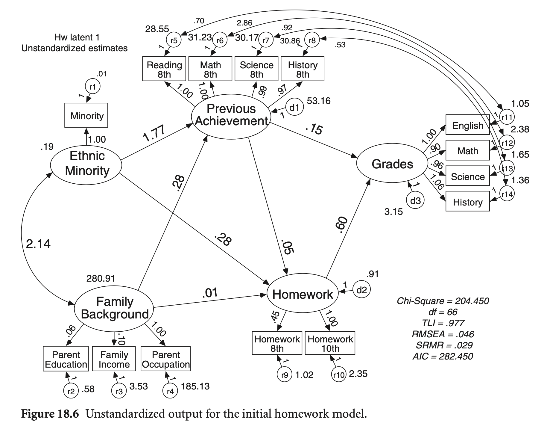
비표준화 결과
어떤 단위로 측정되었는가?
Grades: 0 (an F average) to 12 (A+)
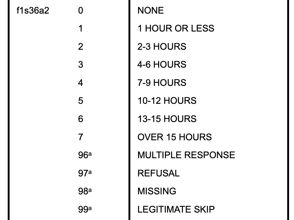
Homework:
소수인종 변수를 통제한 상태에서
All (direct/indirect) paths from family background to grades: total effect
# Using the simulated data
hw_fit_sim <- sem(hw_model, data = hw_sim)library(manymome)
# All indirect paths from family background to grades: total effect
paths <- all_indirect_paths(hw_fit_sim, x = "Famback", y = "Grades")
paths |> print()Call:
all_indirect_paths(fit = hw_fit_sim, x = "Famback", y = "Grades")
Path(s):
path
1 Famback -> PrevAch -> HW -> Grades
2 Famback -> PrevAch -> Grades
3 Famback -> HW -> Grades ind_est_std <- many_indirect_effects(paths,
fit = hw_fit_sim, R = 1000,
boot_ci = TRUE, boot_type = "bc",
standardized_x = TRUE,
standardized_y = TRUE
)
ind_est_std |++++++++++++++++++++++++++++++++++++++++++++++++++| 100% elapsed=16s
==  Indirect Effect(s) (Both x-variable(s) and y-variable(s) Standardized)  ==
                                     std CI.lo CI.hi Sig
Famback -> PrevAch -> HW -> Grades 0.059 0.034 0.108 Sig
Famback -> PrevAch -> Grades       0.284 0.229 0.336 Sig
Famback -> HW -> Grades            0.050 0.013 0.098 Sig

 - [CI.lo to CI.hi] are 95.0% bias-corrected confidence intervals by
   nonparametric bootstrapping with 1000 samples.
 - std: The standardized indirect effects.
# total effect (all indirects + directs) from family background to grades
ind_est_std[[1]] + ind_est_std[[2]] + ind_est_std[[3]]
== Indirect Effect (Both ‘Famback’ and ‘Grades’ Standardized) ==

 Path:                Famback -> PrevAch -> HW -> Grades
 Path:                Famback -> PrevAch -> Grades
 Path:                Famback -> HW -> Grades
 Function of Effects: 0.392
 95.0% Bootstrap CI:  [0.342 to 0.442]

Computation of the Function of Effects:
 ((Famback->PrevAch->HW->Grades)
+(Famback->PrevAch->Grades))
+(Famback->HW->Grades)


Bias-corrected confidence interval formed by nonparametric bootstrapping with
1000 bootstrap samples.
특정 간접효과를 테스트하려면,
indirect_effect(
  fit = hw_fit_sim,
  x = "Famback",
  y = "Grades",
  m = c("HW"),
  boot_out = out_med,
  standardized_x = TRUE,
  standardized_y = TRUE
)

# ==  Indirect Effect(s) (Both x-variable(s) and y-variable(s) Standardized)  ==
#   std CI.lo CI.hi Sig
# famback -> prevach -> hw -> grades 0.060 0.034 0.105 Sig
# famback -> prevach -> grades       0.274 0.222 0.325 Sig
# famback -> hw -> grades            0.054 0.018 0.102 Sig
== Indirect Effect (Both ‘Famback’ and ‘Grades’ Standardized) ==

 Path:            Famback -> HW -> Grades
 Indirect Effect: 0.050

Computation Formula:
  (b.HW~Famback)*(b.Grades~HW)*sd_Famback/sd_Grades

Computation:
  (0.01251)*(0.58685)*(16.70928)/(2.47203)

Coefficients of Component Paths:
       Path Coefficient
 HW~Famback      0.0125
  Grades~HW      0.5868

NOTE:
- The effects of the component paths are from the model, not standardized.가족배경 변수를 통제한 상태에서
All (direct/indirect) paths from minority to grades: total effect
소수인종 변수가 카테고리 변수(더미)이므로 해석에 유의
# All indirect paths from minority to grades: total effect
paths2 <- all_indirect_paths(hw_fit_sim,
  x = "EthnicMinor",
  y = "Grades"
)
paths2 |> print()
Call:
all_indirect_paths(fit = hw_fit_sim, x = "EthnicMinor", y = "Grades")
Path(s):
path
1 EthnicMinor -> PrevAch -> HW -> Grades
2 EthnicMinor -> PrevAch -> Grades
3 EthnicMinor -> HW -> Grades ind_est_std2 <- many_indirect_effects(paths2,
fit = hw_fit_sim, R = 1000,
boot_ci = TRUE, boot_type = "bc",
standardized_x = FALSE, # categorical variable
standardized_y = TRUE
)
ind_est_std2 |++++++++++++++++++++++++++++++++++++++++++++++++++| 100% elapsed=13s
==  Indirect Effect(s) (y-variable(s) Standardized)  ==
                                          ind  CI.lo CI.hi Sig
EthnicMinor -> PrevAch -> HW -> Grades -0.013 -0.040 0.001
EthnicMinor -> PrevAch -> Grades       -0.061 -0.144 0.013
EthnicMinor -> HW -> Grades             0.036 -0.017 0.110

 - [CI.lo to CI.hi] are 95.0% bias-corrected confidence intervals by
   nonparametric bootstrapping with 1000 samples.
 - std: The partially standardized indirect effects.
 - y-variable(s) standardized.
# total effect (all indirects + directs) from minority to grades
ind_est_std2[[1]] + ind_est_std2[[2]] + ind_est_std2[[3]]
== Indirect Effect (‘Grades’ Standardized) ==

 Path:                EthnicMinor -> PrevAch -> HW -> Grades
 Path:                EthnicMinor -> PrevAch -> Grades
 Path:                EthnicMinor -> HW -> Grades
 Function of Effects: -0.037
 95.0% Bootstrap CI:  [-0.146 to 0.073]

Computation of the Function of Effects:
 ((EthnicMinor->PrevAch->HW->Grades)
+(EthnicMinor->PrevAch->Grades))
+(EthnicMinor->HW->Grades)


Bias-corrected confidence interval formed by nonparametric bootstrapping with
1000 bootstrap samples.hw_model_c <- "
EthnicMinor <~ Minority
Famback =~ bypared + byfaminc + parocc
PrevAch =~ bytxrstd + bytxmstd + bytxsstd + bytxhstd
HW =~ hw_8 + hw10
Grades =~ eng_12 + math_12 + sci_12 + ss_12
PrevAch ~ Famback + EthnicMinor
Grades ~ PrevAch + HW
HW ~ PrevAch + Famback + EthnicMinor
"
hw_raw_imp <- VIM::kNN(hw_raw, k = 10) # kNN imputation
csem_fit <- cSEM::csem(.data = hw_raw_imp, .model = hw_model_c, .resample_method = "bootstrap")
cSEM::summarize(csem_fit) |> print()ERROR: Error: 객체 'hw_raw'를 찾을 수 없습니다
Error: 객체 'hw_raw'를 찾을 수 없습니다
Traceback:
1. check_data(data)
2. .handleSimpleError(function (cnd)
. {
. watcher$capture_plot_and_output()
. cnd <- sanitize_call(cnd)
. watcher$push(cnd)
. switch(on_error, continue = invokeRestart("eval_continue"),
. stop = invokeRestart("eval_stop"), error = invokeRestart("eval_error",
. cnd))
. }, "객체 'hw_raw'를 찾을 수 없습니다", base::quote(eval(expr,
. envir)))
# 5. Measurement model
hw_model_cfa <- "
  EthnicMinor =~ Minority
  Famback =~ bypared + byfaminc + parocc
  PrevAch =~ bytxrstd + bytxmstd + bytxsstd + bytxhstd
  HW =~ hw_8 + hw10
  Grades =~ eng_12 + math_12 + sci_12 + ss_12

  Minority ~~ 0.0099*Minority
  bytxrstd ~~ eng_12
  bytxmstd ~~ math_12
  bytxsstd ~~ sci_12
  bytxhstd ~~ ss_12
"
hw_fit_cfa <- cfa(hw_model_cfa, sample.cov = hwcov, sample.nobs = 1000)compareFit(hw_fit, hw_fit_cfa) |> summary() |> print()################### Nested Model Comparison #########################
Chi-Squared Difference Test
Df AIC BIC Chisq Chisq diff RMSEA Df diff Pr(>Chisq)
hw_fit_cfa 64 66742 66944 202.47
hw_fit 66 66741 66932 204.65 2.1889 0.0097196 2 0.3347
####################### Model Fit Indices ###########################
chisq df pvalue rmsea cfi tli srmr aic bic
hw_fit_cfa 202.465† 64 .000 .047 .983† .976 .029† 66742.313 66943.531
hw_fit 204.654 66 .000 .046† .983 .977† .029 66740.502† 66931.905†
################## Differences in Fit Indices #######################
df rmsea cfi tli srmr aic bic
hw_fit - hw_fit_cfa 2 -0.001 0 0.001 0.001 -1.811 -11.627
The following lavaan models were compared:
hw_fit_cfa
hw_fit
To view results, assign the compareFit() output to an object and use the summary() method; see the class?FitDiff help page.Modification indices
modindices(hw_fit, sort = TRUE) |> subset(mi > 10) |> print() lhs op rhs mi epc sepc.lv sepc.all sepc.nox
86 HW =~ bytxmstd 42.221 4.562 2.326 0.223 0.223
98 Grades =~ bytxmstd 37.990 0.734 1.814 0.174 0.174
103 Minority ~~ bypared 23.209 0.067 0.067 0.889 0.889
47 EthnicMinor =~ bypared 22.716 0.395 0.171 0.133 0.133
158 bytxmstd ~~ bytxhstd 21.288 -6.514 -6.514 -0.210 -0.210
48 EthnicMinor =~ byfaminc 18.841 -0.725 -0.314 -0.125 -0.125
104 Minority ~~ byfaminc 18.752 -0.123 -0.123 -0.657 -0.657
99 Grades =~ bytxsstd 14.693 -0.455 -1.123 -0.109 -0.109
167 bytxsstd ~~ eng_12 14.085 -1.009 -1.009 -0.179 -0.179
187 math_12 ~~ sci_12 13.040 0.277 0.277 0.140 0.140
82 HW =~ bypared 11.355 0.358 0.182 0.142 0.142
186 eng_12 ~~ ss_12 10.345 0.285 0.285 0.238 0.238Residuals
Keith’s figure 18.10: normalized residuals
# standardized residuals
resid_z <- residuals(hw_fit, type = "standardized.mplus")$cov
corrplot::corrplot(resid_z, method = 'number', type = 'lower', is.corr = FALSE)
# correlation residuals
resid_cor <- residuals(hw_fit, type = "cor")$cov
corrplot::corrplot(resid_cor, method = 'number', type = 'lower', is.corr = FALSE)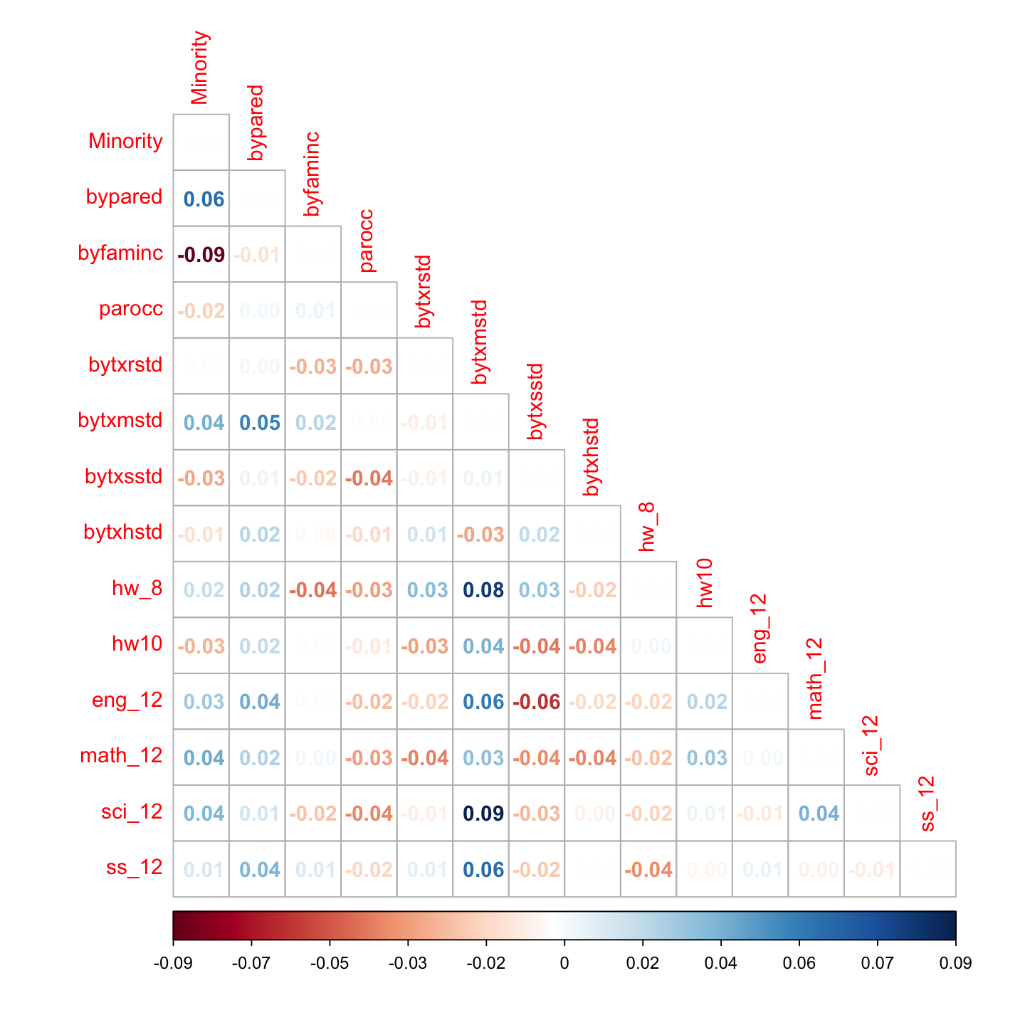
성취도가 locus of control에 미치는 영향과 locus of control이 성취도에 미치는 종단적 영향을 파악하기 위한 모형; 주 목적은 효과의 방향성에 대한 이해
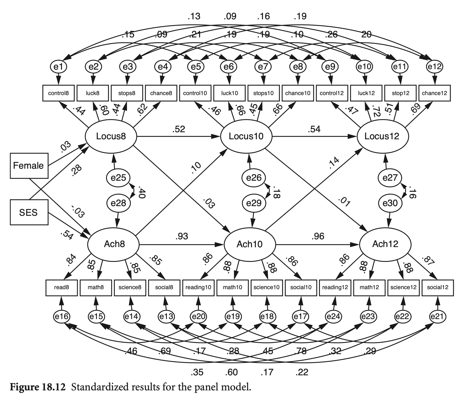
BYS44B 나는 내 인생이 나아가는 방향을 충분히 통제하지 못한다(그림에서 control8)
BYS44C 내 인생에서 성공을 위해서는 노력보다 행운이 더 중요하다(luck8)
BYS44F 내가 앞서 나가려고 할 때마다 무언가 또는 누군가가 나를 막는다 (stops8)
BYS44M 내 인생에서 일어나는 일에는 기회와 행운이 매우 중요하다(chance8)
논의: 각 시점 내에서 인과관계는 설정하지 않았음. Why?
vars <- c("Sex", "BySES", "control8", "luck8", "stops8", "chance8", "contro10", "luck10", "stops10", "chance10", "contro12", "luck12", "stops12", "chance12", "feel8", "worth8", "do8", "sat8", "feel10", "worth10", "do10", "sat10", "feel12", "worth12", "do12", "sat12", "read8", "math8", "scienc8", "social8", "read10", "math10", "scienc10", "social10", "read12", "math12", "scienc12", "social12")
loc_txt <- read_tsv("data/chap 18 latent var SEM 2/sc locus ach matrix n12k.txt", col_names = vars)

loc_mean <- loc_txt[40, ] |> as.double()
loc_sds <- loc_txt[39, ] |> as.double()
loc_cor <- loc_txt[1:38, ] |> as.matrix()
loc_cov <- loc_cor |>
  lav_matrix_vechr(diagonal = TRUE) |>
  getCov(names = vars, sds = loc_sds)
loc_model <- "
# measurement model
Locus8 =~ control8 + luck8 + stops8 + chance8
Locus10 =~ contro10 + luck10 + stops10 + chance10
Locus12 =~ contro12 + luck12 + stops12 + chance12
Ach8 =~ read8 + math8 + scienc8 + social8
Ach10 =~ read10 + math10 + scienc10 + social10
Ach12 =~ read12 + math12 + scienc12 + social12
# structural model
Locus12 ~ Locus10 + Ach10
Ach12 ~ Ach10 + Locus10
Locus10 ~ Locus8 + Ach8
Ach10 ~ Ach8 + Locus8
Locus8 ~ Sex + BySES
Ach8 ~ Sex + BySES
Sex ~~ 0*BySES
# correlated disturbances at each time point
Locus8 ~~ Ach8
Locus10 ~~ Ach10
Locus12 ~~ Ach12
# correlated errors items over time
control8 ~~ contro10
control8 ~~ contro12
contro10 ~~ contro12
luck8 ~~ luck10
luck8 ~~ luck12
luck10 ~~ luck12
stops8 ~~ stops10
stops8 ~~ stops12
stops10 ~~ stops12
chance8 ~~ chance10
chance8 ~~ chance12
chance10 ~~ chance12
read8 ~~ read10
read8 ~~ read12
read10 ~~ read12
math8 ~~ math10
math8 ~~ math12
math10 ~~ math12
scienc8 ~~ scienc10
scienc8 ~~ scienc12
scienc10 ~~ scienc12
social8 ~~ social10
social8 ~~ social12
social10 ~~ social12
"
loc_fit <- sem(loc_model, sample.cov = loc_cov, sample.nobs = 12572)
summary(loc_fit, standardized = TRUE, fit.measures = TRUE) |> print()lavaan 0.6-19 ended normally after 286 iterations
Estimator ML
Optimization method NLMINB
Number of model parameters 89
Number of observations 12572
Model Test User Model:
Test statistic 8204.529
Degrees of freedom 262
P-value (Chi-square) 0.000
Model Test Baseline Model:
Test statistic 224320.606
Degrees of freedom 325
P-value 0.000
User Model versus Baseline Model:
Comparative Fit Index (CFI) 0.965
Tucker-Lewis Index (TLI) 0.956
Loglikelihood and Information Criteria:
Loglikelihood user model (H0) -652454.746
Loglikelihood unrestricted model (H1) -648352.482
Akaike (AIC) 1305087.492
Bayesian (BIC) 1305749.584
Sample-size adjusted Bayesian (SABIC) 1305466.751
Root Mean Square Error of Approximation:
RMSEA 0.049
90 Percent confidence interval - lower 0.048
90 Percent confidence interval - upper 0.050
P-value H_0: RMSEA <= 0.050 0.946
P-value H_0: RMSEA >= 0.080 0.000
Standardized Root Mean Square Residual:
SRMR 0.044
Parameter Estimates:
Standard errors Standard
Information Expected
Information saturated (h1) model Structured
Latent Variables:
Estimate Std.Err z-value P(>|z|) Std.lv Std.all
Locus8 =~
control8 1.000 0.357 0.441
luck8 1.248 0.035 35.417 0.000 0.446 0.605
stops8 0.929 0.030 31.099 0.000 0.332 0.439
chance8 1.555 0.043 35.948 0.000 0.555 0.624
Locus10 =~
contro10 1.000 0.355 0.457
luck10 1.281 0.033 39.181 0.000 0.455 0.663
stops10 0.892 0.027 33.620 0.000 0.317 0.451
chance10 1.459 0.037 39.484 0.000 0.518 0.657
Locus12 =~
contro12 1.000 0.373 0.473
luck12 1.343 0.031 43.051 0.000 0.500 0.719
stops12 0.951 0.025 37.709 0.000 0.354 0.505
chance12 1.489 0.035 43.061 0.000 0.555 0.694
Ach8 =~
read8 1.000 8.564 0.842
math8 1.023 0.008 121.261 0.000 8.763 0.851
scienc8 1.019 0.008 120.649 0.000 8.729 0.855
social8 1.005 0.008 118.952 0.000 8.605 0.846
Ach10 =~
read10 1.000 8.695 0.863
math10 1.021 0.007 136.374 0.000 8.877 0.877
scienc10 1.042 0.008 136.616 0.000 9.064 0.885
social10 1.006 0.008 130.757 0.000 8.744 0.864
Ach12 =~
read12 1.000 8.607 0.857
math12 1.038 0.008 135.026 0.000 8.932 0.883
scienc12 1.036 0.008 133.000 0.000 8.921 0.881
social12 1.016 0.008 130.088 0.000 8.744 0.869
Regressions:
Estimate Std.Err z-value P(>|z|) Std.lv Std.all
Locus12 ~
Locus10 0.564 0.020 28.477 0.000 0.537 0.537
Ach10 0.006 0.000 12.038 0.000 0.136 0.136
Ach12 ~
Ach10 0.950 0.006 151.543 0.000 0.959 0.959
Locus10 0.321 0.107 3.000 0.003 0.013 0.013
Locus10 ~
Locus8 0.521 0.021 24.766 0.000 0.524 0.524
Ach8 0.004 0.001 7.883 0.000 0.103 0.103
Ach10 ~
Ach8 0.945 0.007 132.611 0.000 0.931 0.931
Locus8 0.818 0.142 5.745 0.000 0.034 0.034
Locus8 ~
Sex 0.023 0.008 2.926 0.003 0.063 0.032
BySES 0.126 0.006 22.788 0.000 0.353 0.283
Ach8 ~
Sex -0.540 0.135 -3.994 0.000 -0.063 -0.032
BySES 5.788 0.090 64.430 0.000 0.676 0.542
Covariances:
Estimate Std.Err z-value P(>|z|) Std.lv Std.all
Sex ~~
BySES 0.000 0.000 0.000
.Locus8 ~~
.Ach8 0.982 0.038 25.985 0.000 0.399 0.399
.Locus10 ~~
.Ach10 0.149 0.013 11.154 0.000 0.185 0.185
.Locus12 ~~
.Ach12 0.108 0.011 9.890 0.000 0.160 0.160
.control8 ~~
.contro10 0.077 0.005 15.574 0.000 0.077 0.154
.contro12 0.065 0.005 13.194 0.000 0.065 0.129
.contro10 ~~
.contro12 0.089 0.005 18.824 0.000 0.089 0.186
.luck8 ~~
.luck10 0.026 0.004 7.223 0.000 0.026 0.086
.luck12 0.025 0.003 7.467 0.000 0.025 0.089
.luck10 ~~
.luck12 0.025 0.003 7.839 0.000 0.025 0.101
.stops8 ~~
.stops10 0.089 0.004 21.178 0.000 0.089 0.210
.stops12 0.067 0.004 16.658 0.000 0.067 0.164
.stops10 ~~
.stops12 0.099 0.004 25.969 0.000 0.099 0.263
.chance8 ~~
.chance10 0.076 0.005 15.238 0.000 0.076 0.185
.chance12 0.074 0.005 15.669 0.000 0.074 0.185
.chance10 ~~
.chance12 0.068 0.004 15.871 0.000 0.068 0.199
.read8 ~~
.read10 12.691 0.336 37.725 0.000 12.691 0.456
.read12 9.783 0.327 29.894 0.000 9.783 0.345
.read10 ~~
.read12 11.906 0.319 37.334 0.000 11.906 0.453
.math8 ~~
.math10 18.040 0.351 51.470 0.000 18.040 0.686
.math12 15.389 0.332 46.385 0.000 15.389 0.598
.math10 ~~
.math12 18.056 0.328 55.035 0.000 18.056 0.782
.scienc8 ~~
.scienc10 4.344 0.303 14.353 0.000 4.344 0.171
.scienc12 4.285 0.300 14.284 0.000 4.285 0.168
.scienc10 ~~
.scienc12 7.300 0.290 25.213 0.000 7.300 0.318
.social8 ~~
.social10 7.607 0.323 23.573 0.000 7.607 0.275
.social12 5.962 0.310 19.204 0.000 5.962 0.221
.social10 ~~
.social12 7.351 0.301 24.438 0.000 7.351 0.290
Variances:
Estimate Std.Err z-value P(>|z|) Std.lv Std.all
.control8 0.528 0.008 70.109 0.000 0.528 0.806
.luck8 0.344 0.006 56.216 0.000 0.344 0.634
.stops8 0.460 0.007 70.237 0.000 0.460 0.807
.chance8 0.484 0.009 54.421 0.000 0.484 0.611
.contro10 0.477 0.007 70.646 0.000 0.477 0.791
.luck10 0.264 0.005 51.766 0.000 0.264 0.560
.stops10 0.392 0.006 71.020 0.000 0.392 0.796
.chance10 0.352 0.007 53.246 0.000 0.352 0.568
.contro12 0.482 0.007 71.233 0.000 0.482 0.776
.luck12 0.234 0.005 47.379 0.000 0.234 0.483
.stops12 0.366 0.005 69.721 0.000 0.366 0.745
.chance12 0.331 0.006 51.512 0.000 0.331 0.518
.read8 29.988 0.464 64.565 0.000 29.988 0.290
.math8 29.338 0.461 63.667 0.000 29.338 0.276
.scienc8 28.105 0.454 61.900 0.000 28.105 0.269
.social8 29.485 0.463 63.690 0.000 29.485 0.285
.read10 25.818 0.397 65.026 0.000 25.818 0.255
.math10 23.568 0.372 63.324 0.000 23.568 0.230
.scienc10 22.844 0.377 60.589 0.000 22.844 0.218
.social10 26.025 0.405 64.281 0.000 26.025 0.254
.read12 26.760 0.411 65.092 0.000 26.760 0.265
.math12 22.605 0.369 61.267 0.000 22.605 0.221
.scienc12 23.044 0.380 60.675 0.000 23.044 0.225
.social12 24.674 0.392 62.900 0.000 24.674 0.244
Sex 0.250 0.003 79.284 0.000 0.250 1.000
BySES 0.643 0.008 79.284 0.000 0.643 1.000
.Locus8 0.117 0.006 21.190 0.000 0.919 0.919
.Locus10 0.084 0.004 21.806 0.000 0.664 0.664
.Locus12 0.088 0.004 23.341 0.000 0.636 0.636
.Ach8 51.746 0.913 56.670 0.000 0.705 0.705
.Ach10 7.732 0.194 39.803 0.000 0.102 0.102
.Ach12 5.139 0.139 37.013 0.000 0.069 0.069
카테고리 변수의 레벨에 따라 잠재변수의 효과가 다른지에 대한 검증; 상호작용 효과
연속인 (잠재)변수 간의 상호작용에 대해서는 22장에서 다룸
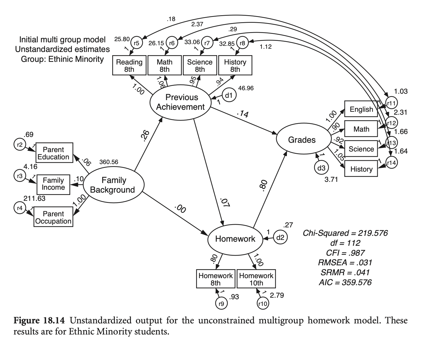
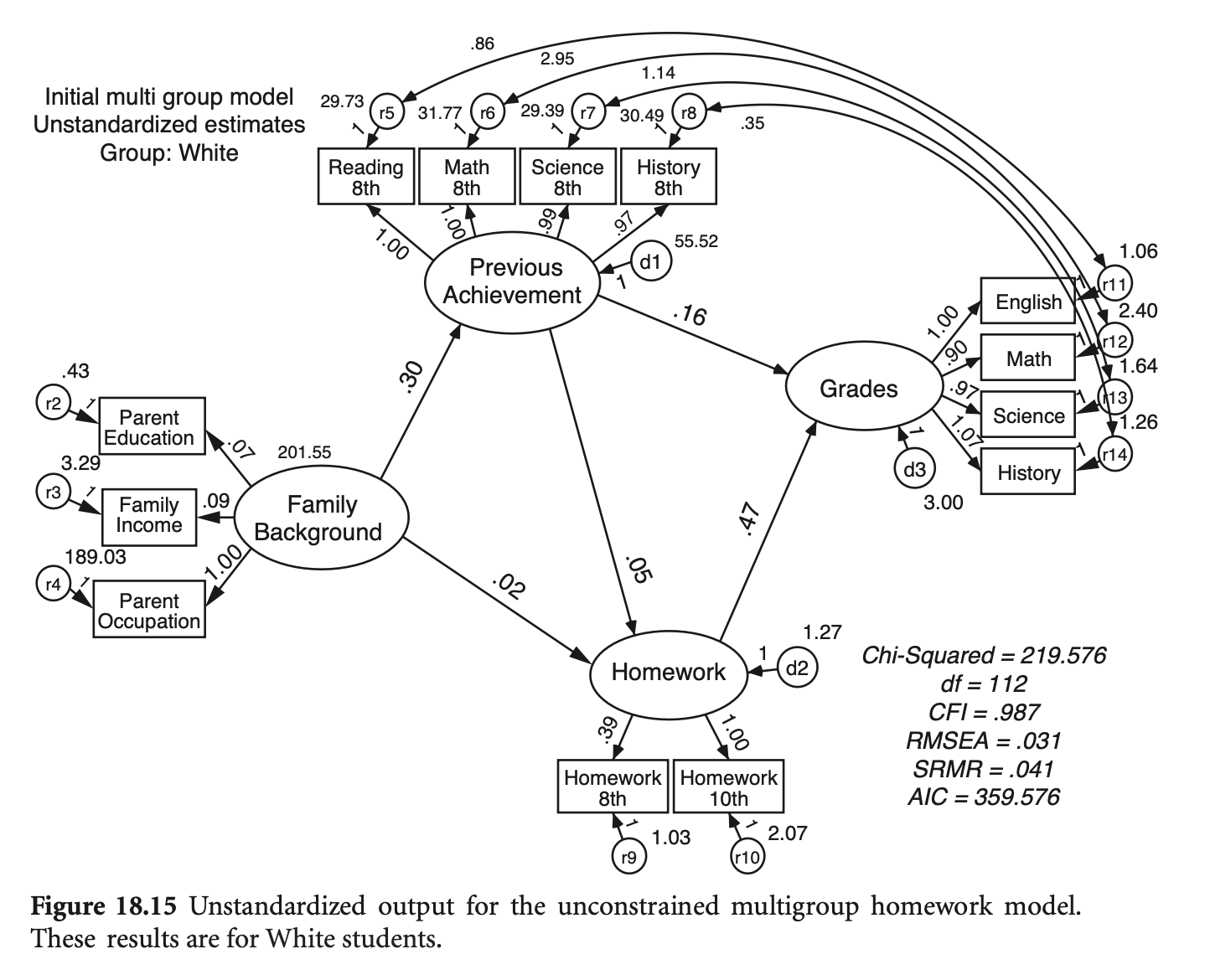
Estimation
그룹별 공분산 행렬로부터 얻어지는 fit function들의 (표본 수) 가중치 평균을 fit function으로 사용
ML estimation의 경우
# generate a dataset with the same covariance matrix
library(readxl)
hw_mg_minor <- read_xls("data/chap 18 latent var SEM 2/minority matrix.xls")
hw_mg_white <- read_xls("data/chap 18 latent var SEM 2/white matrix.xls")

# For minority group
hw_mg_minor_cov <- hw_mg_minor[c(2:14), c(3:15)] |>
  as.matrix() |>
  lav_matrix_vechr(diagonal = TRUE) |>
  getCov(names = hw_mg_minor$varname_[2:14], sds = hw_mg_minor[16, 3:15] |> as.double())
colnames(hw_mg_minor_cov) <- tolower(colnames(hw_mg_minor_cov))
rownames(hw_mg_minor_cov) <- tolower(rownames(hw_mg_minor_cov))
mean_minor <- hw_mg_minor[15, 3:15] |> as.double()

# For white group
hw_mg_white_cov <- hw_mg_white[c(2:14), c(3:15)] |>
  as.matrix() |>
  lav_matrix_vechr(diagonal = TRUE) |>
  getCov(names = hw_mg_white$varname_[2:14], sds = hw_mg_white[16, 3:15] |> as.double())
colnames(hw_mg_white_cov) <- tolower(colnames(hw_mg_white_cov))
rownames(hw_mg_white_cov) <- tolower(rownames(hw_mg_white_cov))
mean_white <- hw_mg_white[15, 3:15] |> as.double()

# simulate the data
set.seed(123) # for reproducibility
hw_sim_minor <- semTools::kd(hw_mg_minor_cov, n = 274, type = "exact") |>
  sweep(2, mean_minor, FUN = "+")
hw_sim_white <- semTools::kd(hw_mg_white_cov, n = 751, type = "exact") |>
  sweep(2, mean_white, FUN = "+")

set.seed(131)
hw_multigroup <- bind_rows(
  hw_sim_minor |> mutate(group = "minority"),
  hw_sim_white |> mutate(group = "white")
) |> sample_n(900)
hw_multigroup |> head() |> print() bypared byfaminc parocc bytxrstd bytxmstd bytxsstd bytxhstd hw_8 hw10
1 3.477102 10.665843 38.43281 46.96390 57.89953 50.71309 45.52944 2.879256 6.703532
2 3.298204 10.055041 46.10124 63.11553 65.43042 46.32358 52.61707 2.718312 5.034043
3 3.392463 9.906801 48.69503 61.66536 62.68831 67.51536 62.09874 2.149325 5.855915
4 2.522122 8.551281 49.65279 56.15432 54.94386 44.65248 47.67488 2.947018 5.570204
5 5.575341 10.891556 64.23261 58.78616 63.80637 57.38648 60.86180 3.403386 4.031776
6 5.192402 10.667251 68.82314 56.87892 54.70169 54.10558 51.51500 5.503236 3.788413
eng_12 math_12 sci_12 ss_12 group
1 8.661664 7.910145 7.247774 8.123688 white
2 6.632333 4.591556 6.289245 7.601705 minority
3 9.070309 5.404964 9.544480 8.503456 minority
4 10.935536 7.104243 9.076028 11.466477 white
5 5.652511 2.516713 3.941772 8.302535 minority
6 7.828620 4.378463 6.640992 8.810365 minorityhw_fit_mg <- sem(hw_model_mg,
sample.cov = list(hw_mg_white_cov, hw_mg_minor_cov),
sample.mean = list(mean_white, mean_minor),
sample.nobs = list(751, 274))Simulated data (N=900)를 이용
# Fit the model
hw_model_mg <- "
  famback =~ parocc + bypared + byfaminc
  prevach =~ bytxrstd + bytxmstd + bytxsstd + bytxhstd
  hw =~ hw10 + hw_8
  grades =~ eng_12 + math_12 + sci_12 + ss_12

  bytxrstd ~~ eng_12
  bytxmstd ~~ math_12
  bytxsstd ~~ sci_12
  bytxhstd ~~ ss_12

  prevach ~ famback
  grades ~ prevach + hw
  hw ~ prevach + famback
"
hw_fit_mg <- sem(hw_model_mg, data = hw_multigroup, group = "group")
summary(hw_fit_mg, standardized = TRUE, fit.measures = TRUE) |> print()
lavaan 0.6-19 ended normally after 402 iterations
Estimator ML
Optimization method NLMINB
Number of model parameters 96
Number of observations per group:
white 665
minority 235
Model Test User Model:
Test statistic 194.017
Degrees of freedom 112
P-value (Chi-square) 0.000
Test statistic for each group:
white 116.568
minority 77.449
Model Test Baseline Model:
Test statistic 7292.337
Degrees of freedom 156
P-value 0.000
User Model versus Baseline Model:
Comparative Fit Index (CFI) 0.989
Tucker-Lewis Index (TLI) 0.984
Loglikelihood and Information Criteria:
Loglikelihood user model (H0) -29423.810
Loglikelihood unrestricted model (H1) -29326.802
Akaike (AIC) 59039.621
Bayesian (BIC) 59500.651
Sample-size adjusted Bayesian (SABIC) 59195.771
Root Mean Square Error of Approximation:
RMSEA 0.040
90 Percent confidence interval - lower 0.031
90 Percent confidence interval - upper 0.050
P-value H_0: RMSEA <= 0.050 0.955
P-value H_0: RMSEA >= 0.080 0.000
Standardized Root Mean Square Residual:
SRMR 0.029
Parameter Estimates:
Standard errors Standard
Information Expected
Information saturated (h1) model Structured
Group 1 [white]:
Latent Variables:
Estimate Std.Err z-value P(>|z|) Std.lv Std.all
famback =~
parocc 1.000 14.608 0.727
bypared 0.071 0.004 15.757 0.000 1.035 0.842
byfaminc 0.096 0.007 13.683 0.000 1.397 0.605
prevach =~
bytxrstd 1.000 8.625 0.849
bytxmstd 0.986 0.037 26.563 0.000 8.509 0.834
bytxsstd 0.967 0.037 26.491 0.000 8.342 0.837
bytxhstd 0.960 0.037 26.134 0.000 8.278 0.834
hw =~
hw10 1.000 1.278 0.660
hw_8 0.381 0.068 5.606 0.000 0.487 0.433
grades =~
eng_12 1.000 2.454 0.924
math_12 0.888 0.030 29.950 0.000 2.179 0.808
sci_12 0.967 0.027 35.958 0.000 2.373 0.879
ss_12 1.062 0.027 39.818 0.000 2.606 0.918
Regressions:
Estimate Std.Err z-value P(>|z|) Std.lv Std.all
prevach ~
famback 0.297 0.028 10.658 0.000 0.504 0.504
grades ~
prevach 0.161 0.012 12.909 0.000 0.567 0.567
hw 0.444 0.120 3.686 0.000 0.231 0.231
hw ~
prevach 0.042 0.010 4.237 0.000 0.285 0.285
famback 0.023 0.006 3.669 0.000 0.259 0.259
Covariances:
Estimate Std.Err z-value P(>|z|) Std.lv Std.all
.bytxrstd ~~
.eng_12 0.862 0.303 2.842 0.004 0.862 0.158
.bytxmstd ~~
.math_12 3.018 0.432 6.985 0.000 3.018 0.337
.bytxsstd ~~
.sci_12 1.349 0.348 3.876 0.000 1.349 0.193
.bytxhstd ~~
.ss_12 0.094 0.328 0.288 0.774 0.094 0.015
Intercepts:
Estimate Std.Err z-value P(>|z|) Std.lv Std.all
.parocc 54.813 0.780 70.297 0.000 54.813 2.726
.bypared 3.321 0.048 69.655 0.000 3.321 2.701
.byfaminc 10.328 0.090 115.341 0.000 10.328 4.473
.bytxrstd 53.051 0.394 134.605 0.000 53.051 5.220
.bytxmstd 53.420 0.396 135.035 0.000 53.420 5.236
.bytxsstd 53.243 0.386 137.807 0.000 53.243 5.344
.bytxhstd 52.914 0.385 137.469 0.000 52.914 5.331
.hw10 3.418 0.075 45.506 0.000 3.418 1.765
.hw_8 1.723 0.044 39.523 0.000 1.723 1.533
.eng_12 6.410 0.103 62.243 0.000 6.410 2.414
.math_12 5.793 0.105 55.391 0.000 5.793 2.148
.sci_12 6.089 0.105 58.201 0.000 6.089 2.257
.ss_12 6.621 0.110 60.106 0.000 6.621 2.331
Variances:
Estimate Std.Err z-value P(>|z|) Std.lv Std.all
.parocc 190.906 15.208 12.553 0.000 190.906 0.472
.bypared 0.441 0.059 7.501 0.000 0.441 0.292
.byfaminc 3.379 0.216 15.625 0.000 3.379 0.634
.bytxrstd 28.897 2.135 13.538 0.000 28.897 0.280
.bytxmstd 31.677 2.252 14.066 0.000 31.677 0.304
.bytxsstd 29.676 2.122 13.983 0.000 29.676 0.299
.bytxhstd 30.003 2.141 14.011 0.000 30.003 0.305
.hw10 2.119 0.310 6.835 0.000 2.119 0.565
.hw_8 1.027 0.071 14.548 0.000 1.027 0.812
.eng_12 1.031 0.090 11.518 0.000 1.031 0.146
.math_12 2.526 0.156 16.171 0.000 2.526 0.347
.sci_12 1.648 0.115 14.386 0.000 1.648 0.226
.ss_12 1.275 0.106 12.025 0.000 1.275 0.158
famback 213.400 22.443 9.509 0.000 1.000 1.000
.prevach 55.537 4.493 12.361 0.000 0.746 0.746
.hw 1.269 0.301 4.213 0.000 0.777 0.777
.grades 3.107 0.232 13.370 0.000 0.516 0.516
Group 2 [minority]:
Latent Variables:
Estimate Std.Err z-value P(>|z|) Std.lv Std.all
famback =~
parocc 1.000 18.455 0.788
bypared 0.057 0.005 10.629 0.000 1.054 0.792
byfaminc 0.105 0.011 9.719 0.000 1.941 0.690
prevach =~
bytxrstd 1.000 8.852 0.877
bytxmstd 1.022 0.058 17.572 0.000 9.046 0.864
bytxsstd 0.897 0.058 15.372 0.000 7.936 0.803
bytxhstd 0.883 0.057 15.505 0.000 7.818 0.804
hw =~
hw10 1.000 0.802 0.442
hw_8 0.731 0.181 4.045 0.000 0.586 0.512
grades =~
eng_12 1.000 2.555 0.936
math_12 0.905 0.047 19.150 0.000 2.312 0.831
sci_12 0.909 0.042 21.428 0.000 2.322 0.875
ss_12 1.037 0.045 22.915 0.000 2.649 0.895
Regressions:
Estimate Std.Err z-value P(>|z|) Std.lv Std.all
prevach ~
famback 0.281 0.037 7.662 0.000 0.587 0.587
grades ~
prevach 0.131 0.042 3.099 0.002 0.455 0.455
hw 0.768 0.603 1.272 0.203 0.241 0.241
hw ~
prevach 0.062 0.015 4.044 0.000 0.681 0.681
famback 0.001 0.006 0.225 0.822 0.031 0.031
Covariances:
Estimate Std.Err z-value P(>|z|) Std.lv Std.all
.bytxrstd ~~
.eng_12 0.257 0.474 0.543 0.587 0.257 0.055
.bytxmstd ~~
.math_12 2.350 0.683 3.441 0.001 2.350 0.288
.bytxsstd ~~
.sci_12 0.287 0.600 0.478 0.632 0.287 0.038
.bytxhstd ~~
.ss_12 1.420 0.629 2.257 0.024 1.420 0.186
Intercepts:
Estimate Std.Err z-value P(>|z|) Std.lv Std.all
.parocc 43.630 1.528 28.555 0.000 43.630 1.863
.bypared 2.823 0.087 32.534 0.000 2.823 2.122
.byfaminc 8.887 0.183 48.462 0.000 8.887 3.161
.bytxrstd 48.458 0.659 73.578 0.000 48.458 4.800
.bytxmstd 49.773 0.683 72.871 0.000 49.773 4.754
.bytxsstd 48.064 0.645 74.522 0.000 48.064 4.861
.bytxhstd 48.249 0.634 76.060 0.000 48.249 4.962
.hw10 3.207 0.118 27.095 0.000 3.207 1.768
.hw_8 1.731 0.075 23.172 0.000 1.731 1.512
.eng_12 5.785 0.178 32.494 0.000 5.785 2.120
.math_12 5.439 0.182 29.961 0.000 5.439 1.954
.sci_12 5.620 0.173 32.455 0.000 5.620 2.117
.ss_12 5.939 0.193 30.769 0.000 5.939 2.007
Variances:
Estimate Std.Err z-value P(>|z|) Std.lv Std.all
.parocc 208.041 31.044 6.701 0.000 208.041 0.379
.bypared 0.658 0.100 6.583 0.000 0.658 0.372
.byfaminc 4.137 0.480 8.621 0.000 4.137 0.523
.bytxrstd 23.579 3.192 7.387 0.000 23.579 0.231
.bytxmstd 27.811 3.569 7.793 0.000 27.811 0.254
.bytxsstd 34.775 3.867 8.994 0.000 34.775 0.356
.bytxhstd 33.441 3.720 8.988 0.000 33.441 0.354
.hw10 2.649 0.305 8.677 0.000 2.649 0.805
.hw_8 0.967 0.132 7.306 0.000 0.967 0.738
.eng_12 0.919 0.152 6.041 0.000 0.919 0.123
.math_12 2.400 0.256 9.370 0.000 2.400 0.310
.sci_12 1.657 0.192 8.631 0.000 1.657 0.235
.ss_12 1.739 0.216 8.063 0.000 1.739 0.199
famback 340.576 52.807 6.449 0.000 1.000 1.000
.prevach 51.378 6.931 7.413 0.000 0.656 0.656
.hw 0.329 0.187 1.762 0.078 0.511 0.511
.grades 3.794 0.484 7.841 0.000 0.581 0.581
두 그룹에게 잠재변수가 동일한 의미를 가지는가?; 20장에서 자세히 다룸
그룹 간에 잠재변수/측정모형의 동일성(invariance)을 검정하기 위해 factor loadings를 그룹 간에 동일하게 제약; (weak invariance)
제약에 대한 lavaan 문법: lavaan 문서
HS.model <- ' visual  =~ x1 + x2 + c(v3,v3)*x3
              textual =~ x4 + x5 + x6
              speed   =~ x7 + x8 + x9 '
또는 다음 예에서 처럼 group.equal = c("loadings") 키워드를 이용
결과표에서 .p1, .p2, …으로 동일하게 제약된 factor loadings를 확인할 수 있음
# contrains factor loadings
hw_fit_mg2 <- sem(hw_model_mg,
  data = hw_multigroup,
  group = "group",
  group.equal = c("loadings")
)
summary(hw_fit_mg2, standardized = TRUE, fit.measures = TRUE) |> print()
lavaan 0.6-19 ended normally after 401 iterations
Estimator ML
Optimization method NLMINB
Number of model parameters 96
Number of equality constraints 9
Number of observations per group:
white 665
minority 235
Model Test User Model:
Test statistic 209.165
Degrees of freedom 121
P-value (Chi-square) 0.000
Test statistic for each group:
white 120.642
minority 88.523
Model Test Baseline Model:
Test statistic 7292.337
Degrees of freedom 156
P-value 0.000
User Model versus Baseline Model:
Comparative Fit Index (CFI) 0.988
Tucker-Lewis Index (TLI) 0.984
Loglikelihood and Information Criteria:
Loglikelihood user model (H0) -29431.384
Loglikelihood unrestricted model (H1) -29326.802
Akaike (AIC) 59036.769
Bayesian (BIC) 59454.577
Sample-size adjusted Bayesian (SABIC) 59178.279
Root Mean Square Error of Approximation:
RMSEA 0.040
90 Percent confidence interval - lower 0.031
90 Percent confidence interval - upper 0.049
P-value H_0: RMSEA <= 0.050 0.963
P-value H_0: RMSEA >= 0.080 0.000
Standardized Root Mean Square Residual:
SRMR 0.033
Parameter Estimates:
Standard errors Standard
Information Expected
Information saturated (h1) model Structured
Group 1 [white]:
Latent Variables:
Estimate Std.Err z-value P(>|z|) Std.lv Std.all
famback =~
parocc 1.000 15.002 0.741
bypared (.p2.) 0.066 0.003 19.026 0.000 0.996 0.819
byfamnc (.p3.) 0.098 0.006 16.614 0.000 1.468 0.628
prevach =~
bytxrst 1.000 8.691 0.851
bytxmst (.p5.) 0.995 0.031 31.773 0.000 8.648 0.840
bytxsst (.p6.) 0.948 0.031 30.716 0.000 8.235 0.833
bytxhst (.p7.) 0.939 0.031 30.463 0.000 8.159 0.829
hw =~
hw10 1.000 1.181 0.613
hw_8 (.p9.) 0.454 0.064 7.059 0.000 0.536 0.473
grades =~
eng_12 1.000 2.467 0.925
math_12 (.11.) 0.893 0.025 35.559 0.000 2.202 0.811
sci_12 (.12.) 0.950 0.023 41.891 0.000 2.344 0.876
ss_12 (.13.) 1.056 0.023 46.042 0.000 2.604 0.917
Regressions:
Estimate Std.Err z-value P(>|z|) Std.lv Std.all
prevach ~
famback 0.293 0.027 11.005 0.000 0.505 0.505
grades ~
prevach 0.160 0.012 12.855 0.000 0.564 0.564
hw 0.480 0.128 3.762 0.000 0.230 0.230
hw ~
prevach 0.041 0.009 4.335 0.000 0.302 0.302
famback 0.021 0.006 3.600 0.000 0.263 0.263
Covariances:
Estimate Std.Err z-value P(>|z|) Std.lv Std.all
.bytxrstd ~~
.eng_12 0.854 0.304 2.813 0.005 0.854 0.157
.bytxmstd ~~
.math_12 2.997 0.432 6.941 0.000 2.997 0.338
.bytxsstd ~~
.sci_12 1.351 0.348 3.884 0.000 1.351 0.191
.bytxhstd ~~
.ss_12 0.117 0.328 0.357 0.721 0.117 0.019
Intercepts:
Estimate Std.Err z-value P(>|z|) Std.lv Std.all
.parocc 54.813 0.785 69.859 0.000 54.813 2.709
.bypared 3.321 0.047 70.439 0.000 3.321 2.732
.byfaminc 10.328 0.091 113.892 0.000 10.328 4.417
.bytxrstd 53.051 0.396 133.951 0.000 53.051 5.194
.bytxmstd 53.420 0.399 133.769 0.000 53.420 5.187
.bytxsstd 53.243 0.384 138.823 0.000 53.243 5.383
.bytxhstd 52.914 0.382 138.555 0.000 52.914 5.373
.hw10 3.418 0.075 45.757 0.000 3.418 1.774
.hw_8 1.723 0.044 39.250 0.000 1.723 1.522
.eng_12 6.410 0.103 61.994 0.000 6.410 2.404
.math_12 5.793 0.105 55.031 0.000 5.793 2.134
.sci_12 6.089 0.104 58.703 0.000 6.089 2.276
.ss_12 6.621 0.110 60.139 0.000 6.621 2.332
Variances:
Estimate Std.Err z-value P(>|z|) Std.lv Std.all
.parocc 184.342 14.742 12.505 0.000 184.342 0.450
.bypared 0.486 0.053 9.178 0.000 0.486 0.329
.byfaminc 3.312 0.215 15.409 0.000 3.312 0.606
.bytxrstd 28.778 2.122 13.559 0.000 28.778 0.276
.bytxmstd 31.265 2.239 13.962 0.000 31.265 0.295
.bytxsstd 29.999 2.109 14.224 0.000 29.999 0.307
.bytxhstd 30.411 2.129 14.283 0.000 30.411 0.314
.hw10 2.317 0.251 9.215 0.000 2.317 0.624
.hw_8 0.994 0.071 14.040 0.000 0.994 0.776
.eng_12 1.023 0.089 11.512 0.000 1.023 0.144
.math_12 2.519 0.156 16.154 0.000 2.519 0.342
.sci_12 1.659 0.114 14.572 0.000 1.659 0.232
.ss_12 1.277 0.105 12.145 0.000 1.277 0.158
famback 225.055 21.210 10.611 0.000 1.000 1.000
.prevach 56.253 4.348 12.938 0.000 0.745 0.745
.hw 1.059 0.229 4.621 0.000 0.759 0.759
.grades 3.140 0.230 13.622 0.000 0.516 0.516
Group 2 [minority]:
Latent Variables:
Estimate Std.Err z-value P(>|z|) Std.lv Std.all
famback =~
parocc 1.000 17.351 0.753
bypared (.p2.) 0.066 0.003 19.026 0.000 1.152 0.841
byfamnc (.p3.) 0.098 0.006 16.614 0.000 1.698 0.625
prevach =~
bytxrst 1.000 8.701 0.872
bytxmst (.p5.) 0.995 0.031 31.773 0.000 8.658 0.847
bytxsst (.p6.) 0.948 0.031 30.716 0.000 8.245 0.817
bytxhst (.p7.) 0.939 0.031 30.463 0.000 8.169 0.821
hw =~
hw10 1.000 0.979 0.530
hw_8 (.p9.) 0.454 0.064 7.059 0.000 0.444 0.396
grades =~
eng_12 1.000 2.523 0.933
math_12 (.11.) 0.893 0.025 35.559 0.000 2.252 0.823
sci_12 (.12.) 0.950 0.023 41.891 0.000 2.397 0.883
ss_12 (.13.) 1.056 0.023 46.042 0.000 2.664 0.897
Regressions:
Estimate Std.Err z-value P(>|z|) Std.lv Std.all
prevach ~
famback 0.295 0.035 8.332 0.000 0.589 0.589
grades ~
prevach 0.118 0.043 2.772 0.006 0.407 0.407
hw 0.826 0.515 1.602 0.109 0.321 0.321
hw ~
prevach 0.068 0.016 4.369 0.000 0.602 0.602
famback 0.006 0.008 0.722 0.470 0.098 0.098
Covariances:
Estimate Std.Err z-value P(>|z|) Std.lv Std.all
.bytxrstd ~~
.eng_12 0.339 0.473 0.717 0.473 0.339 0.071
.bytxmstd ~~
.math_12 2.433 0.689 3.529 0.000 2.433 0.288
.bytxsstd ~~
.sci_12 0.356 0.602 0.591 0.555 0.356 0.048
.bytxhstd ~~
.ss_12 1.376 0.628 2.191 0.028 1.376 0.184
Intercepts:
Estimate Std.Err z-value P(>|z|) Std.lv Std.all
.parocc 43.630 1.503 29.034 0.000 43.630 1.894
.bypared 2.823 0.089 31.592 0.000 2.823 2.061
.byfaminc 8.887 0.177 50.153 0.000 8.887 3.272
.bytxrstd 48.458 0.651 74.428 0.000 48.458 4.855
.bytxmstd 49.773 0.666 74.681 0.000 49.773 4.872
.bytxsstd 48.064 0.659 72.971 0.000 48.064 4.760
.bytxhstd 48.249 0.649 74.326 0.000 48.249 4.849
.hw10 3.207 0.121 26.602 0.000 3.207 1.735
.hw_8 1.731 0.073 23.657 0.000 1.731 1.543
.eng_12 5.785 0.176 32.793 0.000 5.785 2.139
.math_12 5.439 0.179 30.460 0.000 5.439 1.987
.sci_12 5.620 0.177 31.721 0.000 5.620 2.069
.ss_12 5.939 0.194 30.648 0.000 5.939 1.999
Variances:
Estimate Std.Err z-value P(>|z|) Std.lv Std.all
.parocc 229.612 28.952 7.931 0.000 229.612 0.433
.bypared 0.550 0.097 5.667 0.000 0.550 0.293
.byfaminc 4.495 0.472 9.519 0.000 4.495 0.609
.bytxrstd 23.913 3.099 7.716 0.000 23.913 0.240
.bytxmstd 29.426 3.529 8.339 0.000 29.426 0.282
.bytxsstd 33.978 3.820 8.895 0.000 33.978 0.333
.bytxhstd 32.303 3.655 8.837 0.000 32.303 0.326
.hw10 2.457 0.354 6.941 0.000 2.457 0.719
.hw_8 1.060 0.113 9.396 0.000 1.060 0.843
.eng_12 0.946 0.146 6.467 0.000 0.946 0.129
.math_12 2.422 0.255 9.512 0.000 2.422 0.323
.sci_12 1.630 0.191 8.541 0.000 1.630 0.221
.ss_12 1.730 0.212 8.156 0.000 1.730 0.196
famback 301.059 39.678 7.588 0.000 1.000 1.000
.prevach 49.415 6.115 8.081 0.000 0.653 0.653
.hw 0.536 0.281 1.909 0.056 0.558 0.558
.grades 3.562 0.491 7.252 0.000 0.559 0.559
# compare the two models
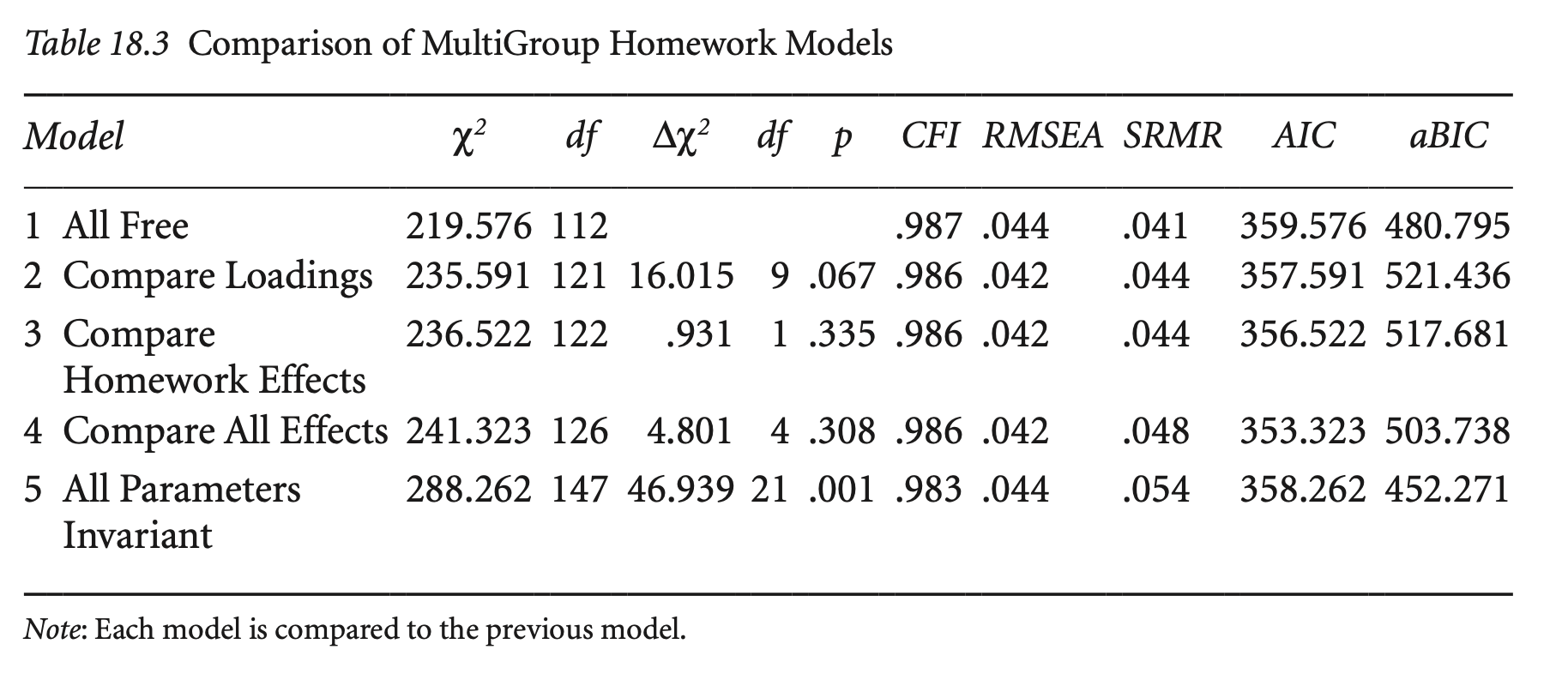
compareFit(hw_fit_mg, hw_fit_mg2) |> summary() |> print()################### Nested Model Comparison #########################
Chi-Squared Difference Test
Df AIC BIC Chisq Chisq diff RMSEA Df diff Pr(>Chisq)
hw_fit_mg 112 59040 59501 194.02
hw_fit_mg2 121 59037 59455 209.16 15.148 0.03896 9 0.08696 .
---
Signif. codes: 0 ‘***’ 0.001 ‘**’ 0.01 ‘*’ 0.05 ‘.’ 0.1 ‘ ’ 1
####################### Model Fit Indices ###########################
chisq df pvalue rmsea cfi tli srmr aic bic
hw_fit_mg 194.017† 112 .000 .040 .989† .984 .029† 59039.621 59500.651
hw_fit_mg2 209.165 121 .000 .040† .988 .984† .033 59036.769† 59454.577†
################## Differences in Fit Indices #######################
df rmsea cfi tli srmr aic bic
hw_fit_mg2 - hw_fit_mg 9 0 -0.001 0 0.004 -2.852 -46.074
The following lavaan models were compared:
hw_fit_mg
hw_fit_mg2
To view results, assign the compareFit() output to an object and use the summary() method; see the class?FitDiff help page.경로 hw → grades가 그룹 간에 동일한가?
# constrains the effect of homework
hw_model_mg3 <- "
  famback =~ parocc + bypared + byfaminc
  prevach =~ bytxrstd + bytxmstd + bytxsstd + bytxhstd
  hw =~ hw10 + hw_8
  grades =~ eng_12 + math_12 + sci_12 + ss_12

  bytxrstd ~~ eng_12
  bytxmstd ~~ math_12
  bytxsstd ~~ sci_12
  bytxhstd ~~ ss_12

  prevach ~ famback
  grades ~ prevach + c(h, h)*hw
  hw ~ prevach + famback
"
hw_fit_mg3 <- sem(hw_model_mg3,
  data = hw_multigroup,
  group = "group",
  group.equal = c("loadings")
)
# compare the models
compareFit(hw_fit_mg, hw_fit_mg2, hw_fit_mg3) |> summary() |> print()################### Nested Model Comparison #########################
Chi-Squared Difference Test
Df AIC BIC Chisq Chisq diff RMSEA Df diff Pr(>Chisq)
hw_fit_mg 112 59040 59501 194.02
hw_fit_mg2 121 59037 59455 209.16 15.1476 0.03896 9 0.08696 .
hw_fit_mg3 122 59035 59448 209.76 0.5932 0.00000 1 0.44117
---
Signif. codes: 0 ‘***’ 0.001 ‘**’ 0.01 ‘*’ 0.05 ‘.’ 0.1 ‘ ’ 1
####################### Model Fit Indices ###########################
chisq df pvalue rmsea cfi tli srmr aic bic
hw_fit_mg 194.017† 112 .000 .040 .989† .984 .029† 59039.621 59500.651
hw_fit_mg2 209.165 121 .000 .040 .988 .984 .033 59036.769 59454.577
hw_fit_mg3 209.758 122 .000 .040† .988 .984† .033 59035.362† 59448.368†
################## Differences in Fit Indices #######################
df rmsea cfi tli srmr aic bic
hw_fit_mg2 - hw_fit_mg 9 0 -0.001 0 0.004 -2.852 -46.074
hw_fit_mg3 - hw_fit_mg2 1 0 0.000 0 0.000 -1.407 -6.209
The following lavaan models were compared:
hw_fit_mg
hw_fit_mg2
hw_fit_mg3
To view results, assign the compareFit() output to an object and use the summary() method; see the class?FitDiff help page.# constrain all the effects
hw_fit_mg4 <- sem(hw_model_mg,
data = hw_multigroup,
group = "group",
group.equal = c("loadings", "regressions")
)# compare the models
compareFit(hw_fit_mg, hw_fit_mg2, hw_fit_mg3, hw_fit_mg4) |> summary() |> print()################### Nested Model Comparison #########################
Chi-Squared Difference Test
Df AIC BIC Chisq Chisq diff RMSEA Df diff Pr(>Chisq)
hw_fit_mg 112 59040 59501 194.02
hw_fit_mg2 121 59037 59455 209.16 15.1476 0.03896 9 0.08696 .
hw_fit_mg3 122 59035 59448 209.76 0.5932 0.00000 1 0.44117
hw_fit_mg4 126 59031 59425 213.11 3.3504 0.00000 4 0.50099
---
Signif. codes: 0 ‘***’ 0.001 ‘**’ 0.01 ‘*’ 0.05 ‘.’ 0.1 ‘ ’ 1
####################### Model Fit Indices ###########################
chisq df pvalue rmsea cfi tli srmr aic bic
hw_fit_mg 194.017† 112 .000 .040 .989† .984 .029† 59039.621 59500.651
hw_fit_mg2 209.165 121 .000 .040 .988 .984 .033 59036.769 59454.577
hw_fit_mg3 209.758 122 .000 .040 .988 .984 .033 59035.362 59448.368
hw_fit_mg4 213.108 126 .000 .039† .988 .985† .034 59030.712† 59424.509†
################## Differences in Fit Indices #######################
df rmsea cfi tli srmr aic bic
hw_fit_mg2 - hw_fit_mg 9 0.000 -0.001 0.000 0.004 -2.852 -46.074
hw_fit_mg3 - hw_fit_mg2 1 0.000 0.000 0.000 0.000 -1.407 -6.209
hw_fit_mg4 - hw_fit_mg3 4 -0.001 0.000 0.001 0.001 -4.650 -23.859
The following lavaan models were compared:
hw_fit_mg
hw_fit_mg2
hw_fit_mg3
hw_fit_mg4
To view results, assign the compareFit() output to an object and use the summary() method; see the class?FitDiff help page.# constrain all the effects & errors
hw_model_mg5 <- "
famback =~ parocc + bypared + byfaminc
prevach =~ bytxrstd + bytxmstd + bytxsstd + bytxhstd
hw =~ hw10 + hw_8
grades =~ eng_12 + math_12 + sci_12 + ss_12
bytxrstd ~~ c(en, en)*eng_12
bytxmstd ~~ c(ma, ma)*math_12
bytxsstd ~~ c(sc, sc)*sci_12
bytxhstd ~~ c(ss, ss)*ss_12
prevach ~ famback
grades ~ prevach + hw
hw ~ prevach + famback
"
hw_fit_mg5 <- sem(hw_model_mg5,
data = hw_multigroup,
group = "group",
group.equal = c(
"loadings", "regressions",
"residuals", "lv.variances"
)
)# compare the models
compareFit(hw_fit_mg, hw_fit_mg2, hw_fit_mg3, hw_fit_mg4, hw_fit_mg5) |> summary() |> print()################### Nested Model Comparison #########################
Chi-Squared Difference Test
Df AIC BIC Chisq Chisq diff RMSEA Df diff Pr(>Chisq)
hw_fit_mg 112 59040 59501 194.02
hw_fit_mg2 121 59037 59455 209.16 15.148 0.03896 9 0.08696 .
hw_fit_mg3 122 59035 59448 209.76 0.593 0.00000 1 0.44117
hw_fit_mg4 126 59031 59425 213.11 3.350 0.00000 4 0.50099
hw_fit_mg5 147 59023 59316 247.26 34.155 0.03731 21 0.03488 *
---
Signif. codes: 0 ‘***’ 0.001 ‘**’ 0.01 ‘*’ 0.05 ‘.’ 0.1 ‘ ’ 1
####################### Model Fit Indices ###########################
chisq df pvalue rmsea cfi tli srmr aic bic
hw_fit_mg 194.017† 112 .000 .040 .989† .984 .029† 59039.621 59500.651
hw_fit_mg2 209.165 121 .000 .040 .988 .984 .033 59036.769 59454.577
hw_fit_mg3 209.758 122 .000 .040 .988 .984 .033 59035.362 59448.368
hw_fit_mg4 213.108 126 .000 .039 .988 .985 .034 59030.712 59424.509
hw_fit_mg5 247.263 147 .000 .039† .986 .985† .044 59022.867† 59315.813†
################## Differences in Fit Indices #######################
df rmsea cfi tli srmr aic bic
hw_fit_mg2 - hw_fit_mg 9 0.000 -0.001 0.000 0.004 -2.852 -46.074
hw_fit_mg3 - hw_fit_mg2 1 0.000 0.000 0.000 0.000 -1.407 -6.209
hw_fit_mg4 - hw_fit_mg3 4 -0.001 0.000 0.001 0.001 -4.650 -23.859
hw_fit_mg5 - hw_fit_mg4 21 0.000 -0.002 0.000 0.010 -7.845 -108.695
The following lavaan models were compared:
hw_fit_mg
hw_fit_mg2
hw_fit_mg3
hw_fit_mg4
hw_fit_mg5
To view results, assign the compareFit() output to an object and use the summary() method; see the class?FitDiff help page.