Load libraries
library(haven)
library(psych)
library(tidyverse)
library(lavaan)
library(semTools)
library(manymome)Multiple Regression and Beyond (3e) by Timothy Z. Keith
library(haven)
library(psych)
library(tidyverse)
library(lavaan)
library(semTools)
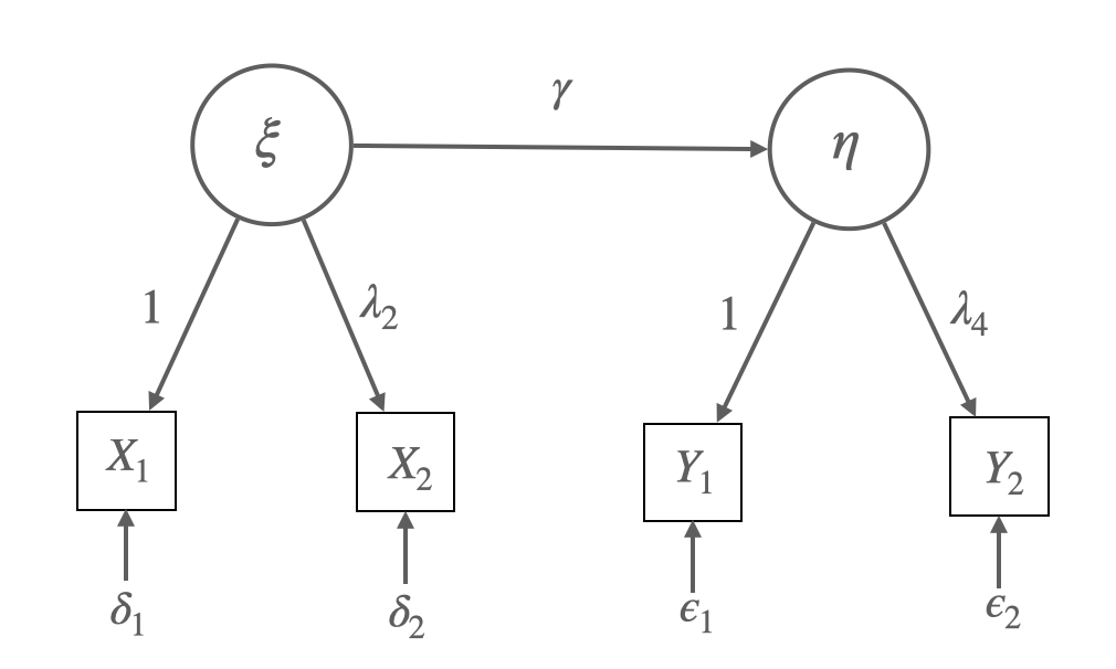
library(manymome)예를 들어, 잠재변수 \(\xi\)가 잠재변수 \(\eta\)에 영향을 주는 모형에 대해,
Structural model:
\(\eta = \alpha + \gamma*\xi + \zeta\)
Measurement model:
\(X_1 = \nu_{X_1} + \xi + \delta_1\)
\(X_2 = \nu_{X_2} + \lambda_{2} *\xi + \delta_2\)
\(Y_1 = \nu_{Y_1} + \eta + \epsilon_1\)
\(Y_2 = \nu_{Y_2} + \lambda_{4}* \eta + \epsilon_2\)
(회귀계수 \(\lambda\): factor loading, 요인부하량, \(\alpha, \nu\): 절편)
각 변수의 평균들은 \(\xi\)의 평균 \(E(\xi) = m\)이라 하면,
\(E(\eta) = \alpha + \gamma*m\),
\(E(X_1) = \nu_{X_1} + m\), \(E(X_2) = \nu_{X_2} + \lambda_{2}*m\),
\(E(Y_1) = \nu_{Y_1} + \alpha + \gamma*m\), \(E(Y_2) = \nu_{Y_2} + \lambda_{4}*(\alpha + \gamma*m)\)
새로운 파라미터 \(m, \alpha, \nu_{X_1}, \nu_{X_2}, \nu_{Y_1}, \nu_{Y_2}\)를 추정하려면, 6개의 정보가 더 필요하나 변수 4개의 평균 정보만 추가되므로 2개의 파라미터의 제약이 필요함.
Multi-group SEM에서 그룹 간에 절편에 대한 동일성을 가정하면, identified 될 수 있음.
변수 \(X\)의 평균의 의미: 예측변수 \(I=(1, 1, ..., 1)\)에 대한 회귀계수인 절편; lm(y ~ 1)
절편(intercept)을 통해 평균(mean)을 추정하게 되고
선형함수에 의해 \(X\)(들)의 평균(벡터)은 \(Y\)의 평균으로 예측됨!
Latent의 평균은 보통 0으로 설정하므로, factor(latent)의 절편은 곧 indicator의 평균이 됨.
파라미터인 절편의 갯수가 늘어나는 만큼 평균에 대한 정보도 늘어나기 때문에,
평균 구조(mean structure)를 추정하더라도 모형의 자유도나 적합도, 모수 등에 변화는 없음.
SEM diagram에서의 표시
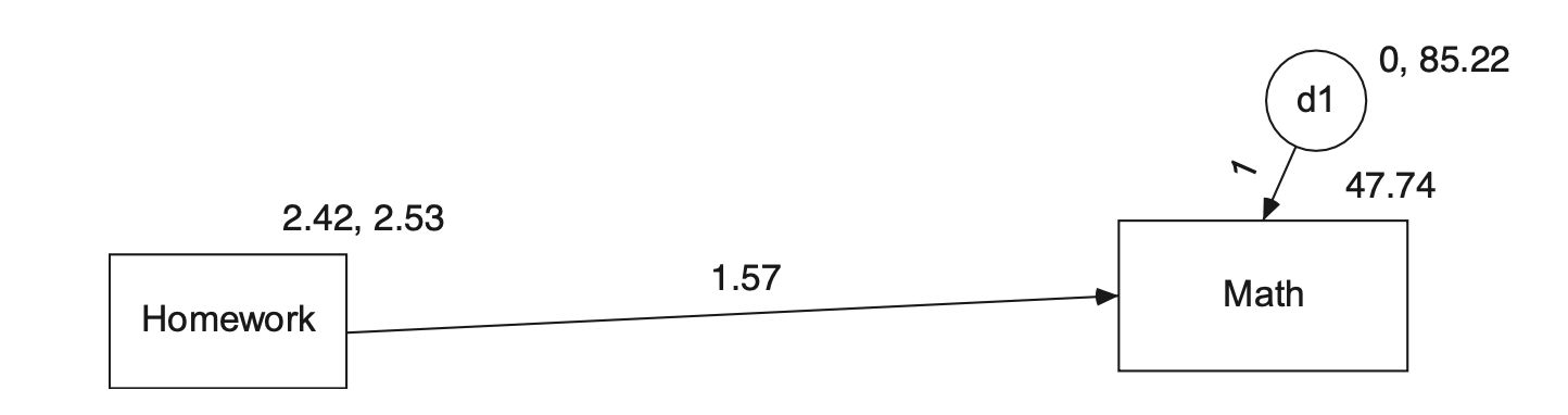
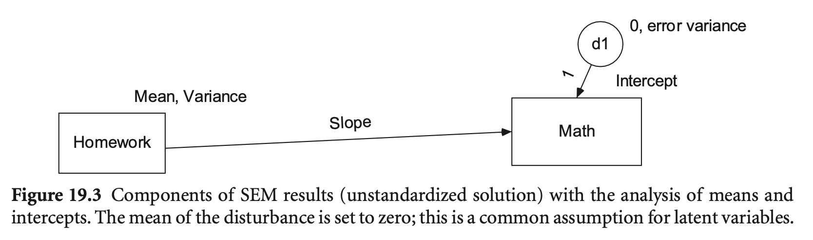
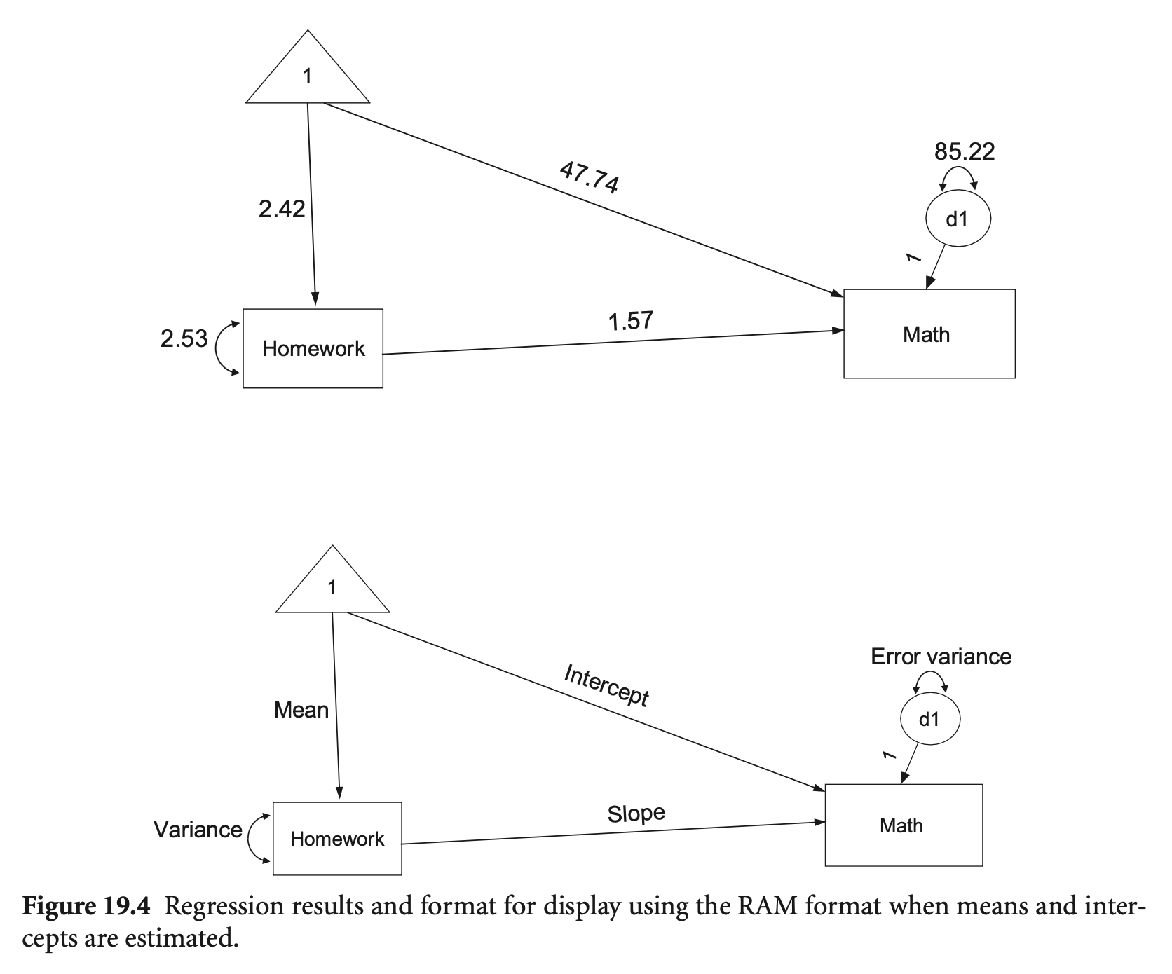
예를 들어,
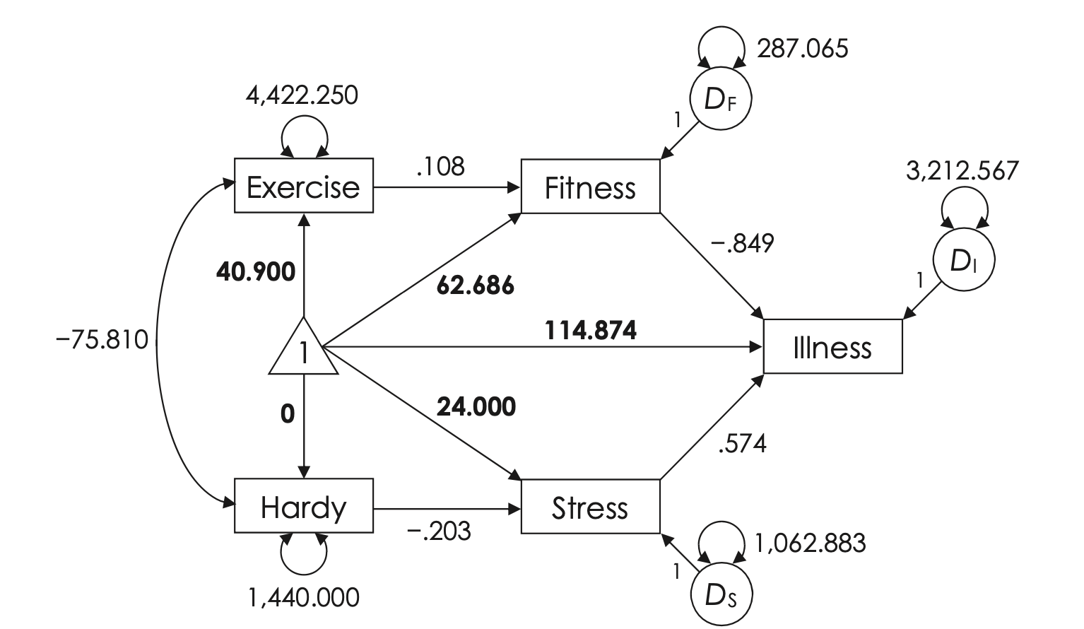
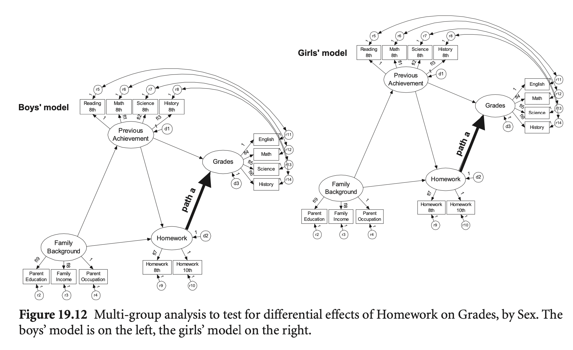
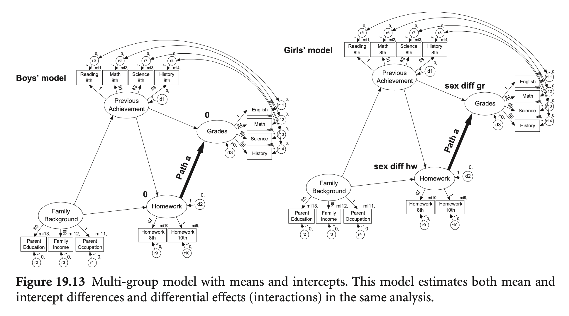
FIGURE 9.1. Recursive path model of illness with unstandardized parameters for the covariance structure and the mean structure. Estimates for the mean structure are shown in boldface. Values for exercise and hardy (exogenous variables) are means, and values for fitness, stress, and illness (endogenous variables) are intercepts.
Source: Kline, R. B. (2023). Principles and practice of structural equation modeling (5e)
hw_mean <- haven::read_sav("data/chap 19 latent means/Homework means.sav")가령, 다음과 같은 모형에 대한 절편을 포함한 파라미터를 추정한다면,
intercept_model <- "
  Grades =~ eng92 + math92 + sci92 + soc92
  HW =~ f2s25f2 + f1s36a2
  Grades ~ HW
"
intercept_fit <- sem(intercept_model, data = hw_mean,  meanstructure = TRUE)
inspect(intercept_fit, what = "estimates") |> print()
$lambda
Grades HW
eng92 1.000 0.000
math92 0.882 0.000
sci92 0.970 0.000
soc92 1.032 0.000
f2s25f2 0.000 1.000
f1s36a2 0.000 1.049
$theta
eng92 math92 sci92 soc92 f2s252 f1s362
eng92 1.052
math92 0.000 2.366
sci92 0.000 0.000 1.494
soc92 0.000 0.000 0.000 1.330
f2s25f2 0.000 0.000 0.000 0.000 2.538
f1s36a2 0.000 0.000 0.000 0.000 0.000 1.407
$psi
Grades HW
Grades 3.671
HW 0.000 1.278
$beta
Grades HW
Grades 0 0.958
HW 0 0.000
$nu
intrcp
eng92 6.512
math92 5.842
sci92 6.163
soc92 6.657
f2s25f2 3.410
f1s36a2 2.584
$alpha
intrcp
Grades 0
HW 0
parameterEstimates(intercept_fit) |> subset(op == "~1") |> print() lhs op rhs est se z pvalue ci.lower ci.upper
16 eng92 ~1 6.512 0.082 79.004 0 6.350 6.673
17 math92 ~1 5.842 0.084 69.495 0 5.677 6.006
18 sci92 ~1 6.163 0.084 73.804 0 6.000 6.327
19 soc92 ~1 6.657 0.086 76.961 0 6.487 6.826
20 f2s25f2 ~1 3.410 0.066 51.434 0 3.280 3.540
21 f1s36a2 ~1 2.584 0.057 45.382 0 2.472 2.696
22 Grades ~1 0.000 0.000 NA NA 0.000 0.000
23 HW ~1 0.000 0.000 NA NA 0.000 0.000summary(intercept_fit,
fit.measures = FALSE,
standardized = TRUE,
remove.unused = FALSE, # keep the unused parameters
) |> print()lavaan 0.6-19 ended normally after 40 iterations
Estimator ML
Optimization method NLMINB
Number of model parameters 19
Used Total
Number of observations 868 1000
Model Test User Model:
Test statistic 20.993
Degrees of freedom 8
P-value (Chi-square) 0.007
Parameter Estimates:
Standard errors Standard
Information Expected
Information saturated (h1) model Structured
Latent Variables:
Estimate Std.Err z-value P(>|z|) Std.lv Std.all
Grades =~
eng92 1.000 2.201 0.906
math92 0.882 0.029 30.161 0.000 1.941 0.784
sci92 0.970 0.026 36.828 0.000 2.135 0.868
soc92 1.032 0.027 38.924 0.000 2.272 0.892
HW =~
f2s25f2 1.000 1.130 0.579
f1s36a2 1.049 0.130 8.089 0.000 1.186 0.707
Regressions:
Estimate Std.Err z-value P(>|z|) Std.lv Std.all
Grades ~
HW 0.958 0.108 8.873 0.000 0.492 0.492
Intercepts:
Estimate Std.Err z-value P(>|z|) Std.lv Std.all
.eng92 6.512 0.082 79.004 0.000 6.512 2.682
.math92 5.842 0.084 69.495 0.000 5.842 2.359
.sci92 6.163 0.084 73.804 0.000 6.163 2.505
.soc92 6.657 0.086 76.961 0.000 6.657 2.612
.f2s25f2 3.410 0.066 51.434 0.000 3.410 1.746
.f1s36a2 2.584 0.057 45.382 0.000 2.584 1.540
.Grades 0.000 0.000 0.000
HW 0.000 0.000 0.000
Variances:
Estimate Std.Err z-value P(>|z|) Std.lv Std.all
.eng92 1.052 0.080 13.149 0.000 1.052 0.178
.math92 2.366 0.130 18.271 0.000 2.366 0.386
.sci92 1.494 0.095 15.780 0.000 1.494 0.247
.soc92 1.330 0.093 14.324 0.000 1.330 0.205
.f2s25f2 2.538 0.195 13.033 0.000 2.538 0.665
.f1s36a2 1.407 0.180 7.798 0.000 1.407 0.500
.Grades 3.671 0.261 14.082 0.000 0.758 0.758
HW 1.278 0.204 6.252 0.000 1.000 1.000
Indicator의 대한 절편을 0으로 고정하고, 잠재변수의 평균을 추정하려면 직접 지정!
intercept_model2 <- "
  Grades =~ eng92 + math92 + sci92 + soc92
  HW =~ f2s25f2 + f1s36a2
  Grades ~ HW

  # specify the intercepts
  Grades ~ 1
  HW ~ 1
  eng92 ~ 0*1
  f2s25f2 ~ 0*1
"
intercept_fit2 <- sem(intercept_model2, data = hw_mean,  meanstructure = TRUE)
inspect(intercept_fit2, what = "estimates") |> print()
$lambda
Grades HW
eng92 1.000 0.000
math92 0.882 0.000
sci92 0.970 0.000
soc92 1.032 0.000
f2s25f2 0.000 1.000
f1s36a2 0.000 1.049
$theta
eng92 math92 sci92 soc92 f2s252 f1s362
eng92 1.052
math92 0.000 2.366
sci92 0.000 0.000 1.494
soc92 0.000 0.000 0.000 1.330
f2s25f2 0.000 0.000 0.000 0.000 2.538
f1s36a2 0.000 0.000 0.000 0.000 0.000 1.407
$psi
Grades HW
Grades 3.671
HW 0.000 1.278
$beta
Grades HW
Grades 0 0.958
HW 0 0.000
$nu
intrcp
eng92 0.000
math92 0.100
sci92 -0.154
soc92 -0.066
f2s25f2 0.000
f1s36a2 -0.995
$alpha
intrcp
Grades 3.244
HW 3.410
summary(intercept_fit2,
  fit.measures = FALSE,
  standardized = TRUE,
  remove.unused = FALSE, # keep the unused parameters
) |> print()
lavaan 0.6-19 ended normally after 63 iterations
Estimator ML
Optimization method NLMINB
Number of model parameters 19
Used Total
Number of observations 868 1000
Model Test User Model:
Test statistic 20.993
Degrees of freedom 8
P-value (Chi-square) 0.007
Parameter Estimates:
Standard errors Standard
Information Expected
Information saturated (h1) model Structured
Latent Variables:
Estimate Std.Err z-value P(>|z|) Std.lv Std.all
Grades =~
eng92 1.000 2.201 0.906
math92 0.882 0.029 30.161 0.000 1.941 0.784
sci92 0.970 0.026 36.828 0.000 2.135 0.868
soc92 1.032 0.027 38.924 0.000 2.272 0.892
HW =~
f2s25f2 1.000 1.130 0.579
f1s36a2 1.049 0.130 8.089 0.000 1.186 0.707
Regressions:
Estimate Std.Err z-value P(>|z|) Std.lv Std.all
Grades ~
HW 0.958 0.108 8.873 0.000 0.492 0.492
Intercepts:
Estimate Std.Err z-value P(>|z|) Std.lv Std.all
.Grades 3.244 0.379 8.555 0.000 1.474 1.474
HW 3.410 0.066 51.434 0.000 3.017 3.017
.eng92 0.000 0.000 0.000
.f2s25f2 0.000 0.000 0.000
.math92 0.100 0.200 0.500 0.617 0.100 0.040
.sci92 -0.154 0.180 -0.857 0.392 -0.154 -0.063
.soc92 -0.066 0.181 -0.367 0.714 -0.066 -0.026
.f1s36a2 -0.995 0.448 -2.221 0.026 -0.995 -0.593
Variances:
Estimate Std.Err z-value P(>|z|) Std.lv Std.all
.eng92 1.052 0.080 13.149 0.000 1.052 0.178
.math92 2.366 0.130 18.271 0.000 2.366 0.386
.sci92 1.494 0.095 15.780 0.000 1.494 0.247
.soc92 1.330 0.093 14.324 0.000 1.330 0.205
.f2s25f2 2.538 0.195 13.033 0.000 2.538 0.665
.f1s36a2 1.407 0.180 7.798 0.000 1.407 0.500
.Grades 3.671 0.261 14.082 0.000 0.758 0.758
HW 1.278 0.204 6.252 0.000 1.000 1.000
Estimation of Means and Intercepts in Single Group SEM Models
hw_model <- "
  Famback =~ parocc + byfaminc + bypared
  Prevach =~ bytxrstd + bytxmstd + bytxsstd + bytxhstd
  HW =~ f2s25f2 + f1s36a2
  Grades =~ eng92 + math92 + sci92 + soc92

  bytxrstd ~~ eng92
  bytxmstd ~~ math92
  bytxsstd ~~ sci92
  bytxhstd ~~ soc92

  Prevach ~ Famback
  Grades ~ Prevach + HW
  HW ~ Prevach + Famback
"
sem_fit <- sem(hw_model,
  data = hw_mean,
  meanstructure = TRUE,
  missing = "FIML"  # for mising data
)
summary(sem_fit, standardized = TRUE, fit.measures = TRUE) |> print()
lavaan 0.6-19 ended normally after 171 iterations
Estimator ML
Optimization method NLMINB
Number of model parameters 48
Number of observations 1000
Number of missing patterns 42
Model Test User Model:
Test statistic 113.358
Degrees of freedom 56
P-value (Chi-square) 0.000
Model Test Baseline Model:
Test statistic 7792.886
Degrees of freedom 78
P-value 0.000
User Model versus Baseline Model:
Comparative Fit Index (CFI) 0.993
Tucker-Lewis Index (TLI) 0.990
Robust Comparative Fit Index (CFI) 0.993
Robust Tucker-Lewis Index (TLI) 0.990
Loglikelihood and Information Criteria:
Loglikelihood user model (H0) -32104.831
Loglikelihood unrestricted model (H1) NA
Akaike (AIC) 64305.662
Bayesian (BIC) 64541.235
Sample-size adjusted Bayesian (SABIC) 64388.784
Root Mean Square Error of Approximation:
RMSEA 0.032
90 Percent confidence interval - lower 0.023
90 Percent confidence interval - upper 0.040
P-value H_0: RMSEA <= 0.050 1.000
P-value H_0: RMSEA >= 0.080 0.000
Robust RMSEA 0.032
90 Percent confidence interval - lower 0.023
90 Percent confidence interval - upper 0.041
P-value H_0: Robust RMSEA <= 0.050 1.000
P-value H_0: Robust RMSEA >= 0.080 0.000
Standardized Root Mean Square Residual:
SRMR 0.023
Parameter Estimates:
Standard errors Standard
Information Observed
Observed information based on Hessian
Latent Variables:
Estimate Std.Err z-value P(>|z|) Std.lv Std.all
Famback =~
parocc 1.000 15.210 0.710
byfaminc 0.124 0.006 19.348 0.000 1.891 0.728
bypared 0.069 0.003 20.632 0.000 1.049 0.834
Prevach =~
bytxrstd 1.000 8.532 0.852
bytxmstd 0.988 0.030 32.651 0.000 8.432 0.853
bytxsstd 0.960 0.031 30.702 0.000 8.189 0.819
bytxhstd 0.942 0.030 31.597 0.000 8.039 0.830
HW =~
f2s25f2 1.000 1.171 0.592
f1s36a2 0.994 0.103 9.671 0.000 1.164 0.688
Grades =~
eng92 1.000 2.436 0.915
math92 0.876 0.025 34.958 0.000 2.135 0.812
sci92 0.961 0.023 41.780 0.000 2.341 0.884
soc92 1.049 0.023 45.416 0.000 2.555 0.908
Regressions:
Estimate Std.Err z-value P(>|z|) Std.lv Std.all
Prevach ~
Famback 0.325 0.022 14.540 0.000 0.579 0.579
Grades ~
Prevach 0.140 0.011 12.973 0.000 0.490 0.490
HW 0.655 0.101 6.491 0.000 0.315 0.315
HW ~
Prevach 0.045 0.008 5.612 0.000 0.331 0.331
Famback 0.018 0.005 3.986 0.000 0.235 0.235
Covariances:
Estimate Std.Err z-value P(>|z|) Std.lv Std.all
.bytxrstd ~~
.eng92 0.486 0.256 1.900 0.057 0.486 0.086
.bytxmstd ~~
.math92 1.573 0.320 4.915 0.000 1.573 0.199
.bytxsstd ~~
.sci92 0.459 0.294 1.563 0.118 0.459 0.064
.bytxhstd ~~
.soc92 0.266 0.278 0.956 0.339 0.266 0.042
Intercepts:
Estimate Std.Err z-value P(>|z|) Std.lv Std.all
.parocc 51.388 0.679 75.669 0.000 51.388 2.400
.byfaminc 9.841 0.083 118.414 0.000 9.841 3.792
.bypared 3.128 0.040 78.568 0.000 3.128 2.485
.bytxrstd 51.257 0.320 160.386 0.000 51.257 5.120
.bytxmstd 51.493 0.316 163.072 0.000 51.493 5.206
.bytxsstd 51.179 0.320 160.149 0.000 51.179 5.117
.bytxhstd 51.373 0.310 165.931 0.000 51.373 5.302
.f2s25f2 3.280 0.066 49.942 0.000 3.280 1.659
.f1s36a2 2.481 0.055 45.366 0.000 2.481 1.465
.eng92 6.074 0.084 71.892 0.000 6.074 2.281
.math92 5.482 0.083 65.676 0.000 5.482 2.086
.sci92 5.770 0.084 68.653 0.000 5.770 2.177
.soc92 6.207 0.089 69.614 0.000 6.207 2.207
Variances:
Estimate Std.Err z-value P(>|z|) Std.lv Std.all
.parocc 227.271 13.266 17.132 0.000 227.271 0.496
.byfaminc 3.161 0.198 15.973 0.000 3.161 0.469
.bypared 0.483 0.044 10.967 0.000 0.483 0.305
.bytxrstd 27.413 1.704 16.091 0.000 27.413 0.274
.bytxmstd 26.728 1.669 16.017 0.000 26.728 0.273
.bytxsstd 32.977 1.881 17.536 0.000 32.977 0.330
.bytxhstd 29.242 1.709 17.107 0.000 29.242 0.312
.f2s25f2 2.537 0.178 14.290 0.000 2.537 0.649
.f1s36a2 1.510 0.149 10.158 0.000 1.510 0.527
.eng92 1.155 0.080 14.479 0.000 1.155 0.163
.math92 2.349 0.122 19.249 0.000 2.349 0.340
.sci92 1.541 0.092 16.744 0.000 1.541 0.219
.soc92 1.383 0.091 15.197 0.000 1.383 0.175
Famback 231.337 19.948 11.597 0.000 1.000 1.000
.Prevach 48.379 3.317 14.583 0.000 0.665 0.665
.HW 1.021 0.154 6.644 0.000 0.745 0.745
.Grades 3.063 0.200 15.324 0.000 0.516 0.516
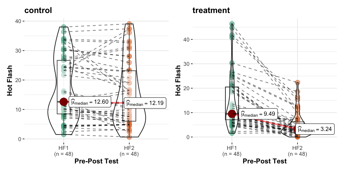
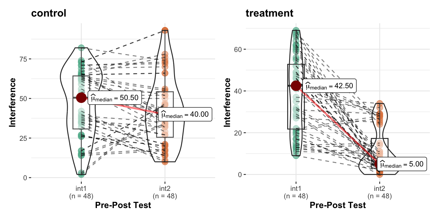
Elkins et. al. (2008). Randomized trial of a hypnosis intervention for treatment of hot flashes among breast cancer survivors. Journal of Clinical Oncology, 26(31), 5022-5026.
# load the dataset
hotflash <- read_sav("data/chap 19 latent means/hot flash simulated.sav")
# make a grouping variable as a factor
hotflash <- hotflash |>
  mutate(g = factor(Group, labels = c("control", "treatment")))
hotflash |> print()
# A tibble: 96 × 6
Group HF1 HF2 int1 int2 g
<dbl+lbl> <dbl> <dbl> <dbl> <dbl> <fct>
1 0 [Control] 33.4 32.7 64 38 control
2 1 [Hypnosis Intervention] 25.5 12.7 52 5 treatment
3 1 [Hypnosis Intervention] 11.0 7.60 9 2 treatment
4 1 [Hypnosis Intervention] 8.05 4.05 13 6 treatment
5 0 [Control] 13.2 4.34 61 36 control
6 0 [Control] 9.89 8.89 15 34 control
# ℹ 90 more rowsggstatsplot을 이용해 시각화
모형에 대한 가정 검토
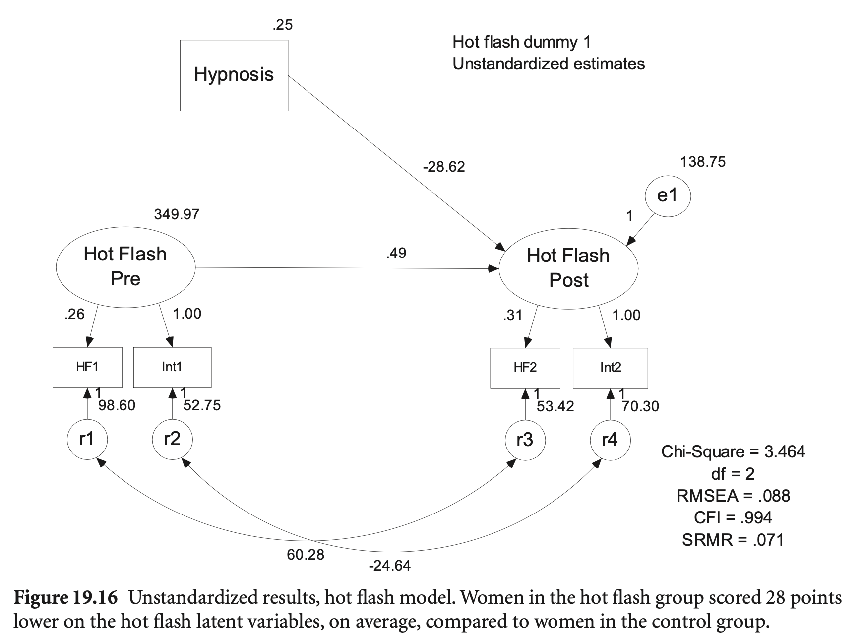
hotflash_model <- "
  hf_pre =~ int1 + HF1
  hf_post =~ int2 + HF2

  hf_post ~ hf_pre + Group  # Group: numeric variable!

  HF1 ~~ HF2
  int1 ~~ int2
"
hotflash_fit <- sem(hotflash_model, data = hotflash)
summary(hotflash_fit,
  standardized = "std.nox", # dummy 변수에 대해서는 표준화하지 않기 위함
  fit.measures = TRUE) |> print()
lavaan 0.6-19 ended normally after 161 iterations
Estimator ML
Optimization method NLMINB
Number of model parameters 12
Number of observations 96
Model Test User Model:
Test statistic 3.501
Degrees of freedom 2
P-value (Chi-square) 0.174
Model Test Baseline Model:
Test statistic 244.790
Degrees of freedom 10
P-value 0.000
User Model versus Baseline Model:
Comparative Fit Index (CFI) 0.994
Tucker-Lewis Index (TLI) 0.968
Loglikelihood and Information Criteria:
Loglikelihood user model (H0) -1466.241
Loglikelihood unrestricted model (H1) NA
Akaike (AIC) 2956.482
Bayesian (BIC) 2987.254
Sample-size adjusted Bayesian (SABIC) 2949.365
Root Mean Square Error of Approximation:
RMSEA 0.088
90 Percent confidence interval - lower 0.000
90 Percent confidence interval - upper 0.239
P-value H_0: RMSEA <= 0.050 0.245
P-value H_0: RMSEA >= 0.080 0.649
Standardized Root Mean Square Residual:
SRMR 0.082
Parameter Estimates:
Standard errors Standard
Information Expected
Information saturated (h1) model Structured
Latent Variables:
Estimate Std.Err z-value P(>|z|) Std.nox
hf_pre =~
int1 1.000 0.932
HF1 0.260 0.112 2.323 0.020 0.439
hf_post =~
int2 1.000 0.927
HF2 0.310 0.037 8.480 0.000 0.659
Regressions:
Estimate Std.Err z-value P(>|z|) Std.nox
hf_post ~
hf_pre 0.487 0.195 2.500 0.012 0.441
Group -28.615 3.149 -9.087 0.000 -1.386
Covariances:
Estimate Std.Err z-value P(>|z|) Std.nox
.HF1 ~~
.HF2 60.277 10.820 5.571 0.000 0.831
.int1 ~~
.int2 -24.643 55.046 -0.448 0.654 -0.405
Variances:
Estimate Std.Err z-value P(>|z|) Std.nox
.int1 52.754 179.207 0.294 0.768 0.131
.HF1 98.604 17.851 5.524 0.000 0.807
.int2 70.301 51.321 1.370 0.171 0.142
.HF2 53.415 9.107 5.865 0.000 0.565
hf_pre 349.972 190.044 1.842 0.066 1.000
.hf_post 138.752 35.569 3.901 0.000 0.325
# free covariance between pretest and group
hotflash_model2 <- "
  hf_pre =~ int1 + HF1
  hf_post =~ int2 + HF2

  hf_post ~ hf_pre + Group
  hf_pre ~ Group  # free the parameter

  HF1 ~~ HF2
  int1 ~~ int2

  # 또는 hf_pre ~~ Group
"
hotflash_fit2 <- sem(hotflash_model2, data = hotflash)
parameterEstimates(hotflash_fit2, standardized = TRUE) |> subset(rhs == "Group") |> print()
lhs op rhs est se z pvalue ci.lower ci.upper std.lv std.all std.nox
6 hf_post ~ Group -27.460 3.413 -8.047 0.00 -34.149 -20.771 -1.286 -0.643 -1.286
7 hf_pre ~ Group -7.485 3.982 -1.880 0.06 -15.289 0.318 -0.428 -0.214 -0.428
16 Group ~~ Group 0.250 0.000 NA NA 0.250 0.250 0.250 1.000 0.250lavTestLRT(hotflash_fit2, hotflash_fit) |> print()
Chi-Squared Difference Test

              Df    AIC    BIC  Chisq Chisq diff   RMSEA Df diff Pr(>Chisq)
hotflash_fit2  1 2955.1 2988.4 0.0881
hotflash_fit   2 2956.5 2987.2 3.5007     3.4126 0.15853       1     0.0647 .
---
Signif. codes:  0 ‘***’ 0.001 ‘**’ 0.01 ‘*’ 0.05 ‘.’ 0.1 ‘ ’ 1
# no effect of group on post-test
hotflash_model3 <- "
hf_pre =~ int1 + HF1
hf_post =~ int2 + HF2
hf_post ~ hf_pre + 0*Group # fix the parameter to 0
hf_pre ~ Group # free the parameter
HF1 ~~ HF2
int1 ~~ int2
"
hotflash_fit3 <- sem(hotflash_model3, data = hotflash)compareFit(hotflash_fit3, hotflash_fit2) |> summary() |> print()################### Nested Model Comparison #########################
Chi-Squared Difference Test
Df AIC BIC Chisq Chisq diff RMSEA Df diff Pr(>Chisq)
hotflash_fit2 1 2955.1 2988.4 0.0881
hotflash_fit3 2 2969.2 3000.0 16.2486 16.16 0.39739 1 5.82e-05 ***
---
Signif. codes: 0 ‘***’ 0.001 ‘**’ 0.01 ‘*’ 0.05 ‘.’ 0.1 ‘ ’ 1
####################### Model Fit Indices ###########################
chisq df pvalue rmsea cfi tli srmr aic bic
hotflash_fit2 .088† 1 .767 .000† 1.000† 1.039† .009† 2955.070† 2988.406†
hotflash_fit3 16.249 2 .000 .272 .939 .697 .113 2969.230 3000.002
################## Differences in Fit Indices #######################
df rmsea cfi tli srmr aic bic
hotflash_fit3 - hotflash_fit2 1 0.272 -0.061 -0.342 0.104 14.16 11.596
The following lavaan models were compared:
hotflash_fit2
hotflash_fit3
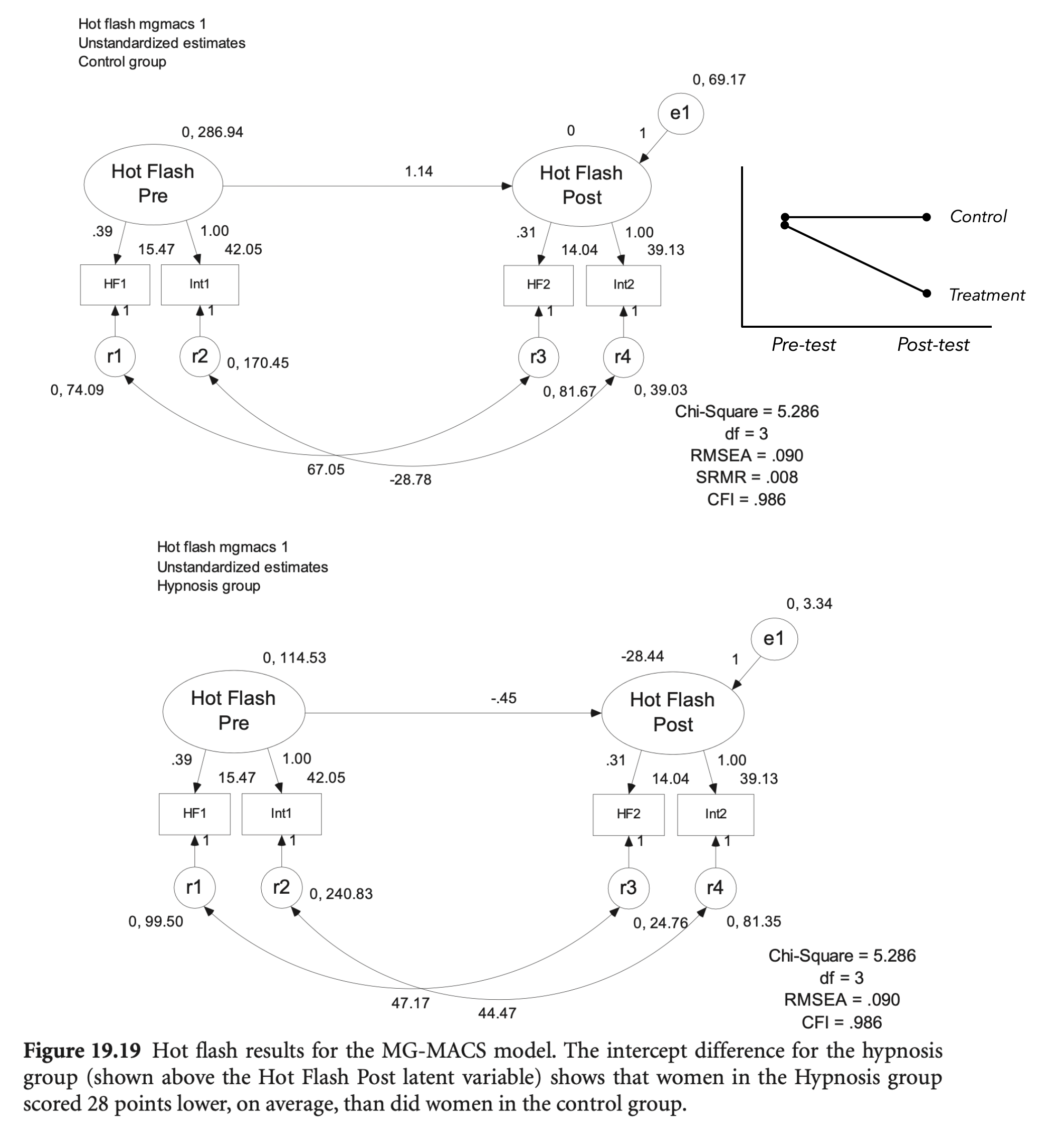
To view results, assign the compareFit() output to an object and use the summary() method; see the class?FitDiff help page.MG-MACS (Multiple Group Mean and Covariance Structure Analysis) Approach
측정 모형에 대해서:
구조 모형에 대해서:
# initial model
hotflash_model_mg <- "
  hf_pre =~ int1 + HF1
  hf_post =~ int2 + HF2

  hf_post ~ hf_pre

  HF1 ~~ HF2
  int1 ~~ int2

  hf_pre ~ 0*1  # default로 group2에서 intercept를 0으로 고정하지 않음!

  ### Defaults
  # hf_post ~ c(a1, a2)*1  # 첫번째 집단의 intercept:0, 두번째 집단 intercept는 추정
  # a1 == 0
"
hotflash_fit_mg <- sem(hotflash_model_mg,
  data = hotflash,
  meanstructure = TRUE, # mean structure
  group = "g", # factor type
  group.equal = c("loadings", "intercepts")
)
summary(hotflash_fit_mg,
  standardized = TRUE,
  fit.measures = TRUE,
  remove.unused = FALSE, # keep the unused parameters
) |> print()
lavaan 0.6-19 ended normally after 326 iterations
Estimator ML
Optimization method NLMINB
Number of model parameters 31
Number of equality constraints 6
Number of observations per group:
control 48
treatment 48
Model Test User Model:
Test statistic 5.399
Degrees of freedom 3
P-value (Chi-square) 0.145
Test statistic for each group:
control 2.169
treatment 3.229
Model Test Baseline Model:
Test statistic 182.941
Degrees of freedom 12
P-value 0.000
User Model versus Baseline Model:
Comparative Fit Index (CFI) 0.986
Tucker-Lewis Index (TLI) 0.944
Loglikelihood and Information Criteria:
Loglikelihood user model (H0) -1425.733
Loglikelihood unrestricted model (H1) -1423.033
Akaike (AIC) 2901.465
Bayesian (BIC) 2965.574
Sample-size adjusted Bayesian (SABIC) 2886.638
Root Mean Square Error of Approximation:
RMSEA 0.129
90 Percent confidence interval - lower 0.000
90 Percent confidence interval - upper 0.302
P-value H_0: RMSEA <= 0.050 0.185
P-value H_0: RMSEA >= 0.080 0.751
Standardized Root Mean Square Residual:
SRMR 0.088
Parameter Estimates:
Standard errors Standard
Information Expected
Information saturated (h1) model Structured
Group 1 [control]:
Latent Variables:
Estimate Std.Err z-value P(>|z|) Std.lv Std.all
hf_pre =~
int1 1.000 16.945 0.792
HF1 (.p2.) 0.388 0.115 3.388 0.001 6.573 0.607
hf_post =~
int2 1.000 21.010 0.959
HF2 (.p4.) 0.312 0.037 8.433 0.000 6.559 0.587
Regressions:
Estimate Std.Err z-value P(>|z|) Std.lv Std.all
hf_post ~
hf_pre 1.139 0.274 4.156 0.000 0.919 0.919
Covariances:
Estimate Std.Err z-value P(>|z|) Std.lv Std.all
.HF1 ~~
.HF2 67.058 18.003 3.725 0.000 67.058 0.862
.int1 ~~
.int2 -28.916 98.630 -0.293 0.769 -28.916 -0.355
Intercepts:
Estimate Std.Err z-value P(>|z|) Std.lv Std.all
hf_pre 0.000 0.000 0.000
.int1 (.15.) 42.049 2.027 20.742 0.000 42.049 1.966
.HF1 (.16.) 15.473 1.089 14.206 0.000 15.473 1.429
.int2 (.17.) 39.131 2.690 14.548 0.000 39.131 1.785
.HF2 (.18.) 14.044 1.248 11.256 0.000 14.044 1.258
.hf_post 0.000 0.000 0.000
Variances:
Estimate Std.Err z-value P(>|z|) Std.lv Std.all
.int1 170.287 124.805 1.364 0.172 170.287 0.372
.HF1 74.107 19.536 3.793 0.000 74.107 0.632
.int2 39.030 107.473 0.363 0.716 39.030 0.081
.HF2 81.674 19.666 4.153 0.000 81.674 0.655
hf_pre 287.136 148.917 1.928 0.054 1.000 1.000
.hf_post 68.950 49.956 1.380 0.168 0.156 0.156
Group 2 [treatment]:
Latent Variables:
Estimate Std.Err z-value P(>|z|) Std.lv Std.all
hf_pre =~
int1 1.000 10.689 0.567
HF1 (.p2.) 0.388 0.115 3.388 0.001 4.146 0.384
hf_post =~
int2 1.000 5.158 0.496
HF2 (.p4.) 0.312 0.037 8.433 0.000 1.610 0.308
Regressions:
Estimate Std.Err z-value P(>|z|) Std.lv Std.all
hf_post ~
hf_pre -0.456 0.459 -0.993 0.321 -0.944 -0.944
Covariances:
Estimate Std.Err z-value P(>|z|) Std.lv Std.all
.HF1 ~~
.HF2 47.191 10.578 4.461 0.000 47.191 0.950
.int1 ~~
.int2 44.760 37.540 1.192 0.233 44.760 0.319
Intercepts:
Estimate Std.Err z-value P(>|z|) Std.lv Std.all
hf_pre 0.000 0.000 0.000
.int1 (.15.) 42.049 2.027 20.742 0.000 42.049 2.230
.HF1 (.16.) 15.473 1.089 14.206 0.000 15.473 1.432
.int2 (.17.) 39.131 2.690 14.548 0.000 39.131 3.764
.HF2 (.18.) 14.044 1.248 11.256 0.000 14.044 2.684
.hf_post -28.439 3.135 -9.071 0.000 -5.513 -5.513
Variances:
Estimate Std.Err z-value P(>|z|) Std.lv Std.all
.int1 241.229 74.588 3.234 0.001 241.229 0.679
.HF1 99.551 23.596 4.219 0.000 99.551 0.853
.int2 81.492 25.448 3.202 0.001 81.492 0.754
.HF2 24.780 5.610 4.417 0.000 24.780 0.905
hf_pre 114.255 70.087 1.630 0.103 1.000 1.000
.hf_post 2.901 52.283 0.055 0.956 0.109 0.109
parameterEstimates(hotflash_fit_mg) |> subset(op == "~1") |> print() lhs op rhs block group label est se z pvalue ci.lower ci.upper
8 hf_pre ~1 1 1 0.000 0.000 NA NA 0.000 0.000
15 int1 ~1 1 1 .p15. 42.049 2.027 20.742 0 38.075 46.022
16 HF1 ~1 1 1 .p16. 15.473 1.089 14.206 0 13.339 17.608
17 int2 ~1 1 1 .p17. 39.131 2.690 14.548 0 33.859 44.403
18 HF2 ~1 1 1 .p18. 14.044 1.248 11.256 0 11.598 16.489
19 hf_post ~1 1 1 0.000 0.000 NA NA 0.000 0.000
27 hf_pre ~1 2 2 0.000 0.000 NA NA 0.000 0.000
34 int1 ~1 2 2 .p15. 42.049 2.027 20.742 0 38.075 46.022
35 HF1 ~1 2 2 .p16. 15.473 1.089 14.206 0 13.339 17.608
36 int2 ~1 2 2 .p17. 39.131 2.690 14.548 0 33.859 44.403
37 HF2 ~1 2 2 .p18. 14.044 1.248 11.256 0 11.598 16.489
38 hf_post ~1 2 2 -28.439 3.135 -9.071 0 -34.584 -22.295# Free parameters 확인
parTable(hotflash_fit_mg) |> print() id lhs op rhs user block group free ustart exo label plabel start est
1 1 hf_pre =~ int1 1 1 1 0 1 0 .p1. 1.000 1.000
2 2 hf_pre =~ HF1 1 1 1 1 NA 0 .p2. .p2. 0.388 0.388
3 3 hf_post =~ int2 1 1 1 0 1 0 .p3. 1.000 1.000
4 4 hf_post =~ HF2 1 1 1 2 NA 0 .p4. .p4. 0.448 0.312
5 5 hf_post ~ hf_pre 1 1 1 3 NA 0 .p5. 0.000 1.139
6 6 HF1 ~~ HF2 1 1 1 4 NA 0 .p6. 0.000 67.058
7 7 int1 ~~ int2 1 1 1 5 NA 0 .p7. 0.000 -28.916
8 8 hf_pre ~1 1 1 1 0 0 0 .p8. 0.000 0.000
9 9 int1 ~~ int1 0 1 1 6 NA 0 .p9. 224.087 170.287
10 10 HF1 ~~ HF1 0 1 1 7 NA 0 .p10. 57.344 74.107
11 11 int2 ~~ int2 0 1 1 8 NA 0 .p11. 233.573 39.030
12 12 HF2 ~~ HF2 0 1 1 9 NA 0 .p12. 61.474 81.674
13 13 hf_pre ~~ hf_pre 0 1 1 10 NA 0 .p13. 0.050 287.136
14 14 hf_post ~~ hf_post 0 1 1 11 NA 0 .p14. 0.050 68.950
15 15 int1 ~1 0 1 1 12 NA 0 .p15. .p15. 46.312 42.049
16 16 HF1 ~1 0 1 1 13 NA 0 .p16. .p16. 17.077 15.473
17 17 int2 ~1 0 1 1 14 NA 0 .p17. .p17. 42.250 39.131
18 18 HF2 ~1 0 1 1 15 NA 0 .p18. .p18. 15.508 14.044
19 19 hf_post ~1 0 1 1 0 0 0 .p19. 0.000 0.000
20 20 hf_pre =~ int1 1 2 2 0 1 0 .p20. 1.000 1.000
21 21 hf_pre =~ HF1 1 2 2 16 NA 0 .p2. .p21. 0.275 0.388
22 22 hf_post =~ int2 1 2 2 0 1 0 .p22. 1.000 1.000
23 23 hf_post =~ HF2 1 2 2 17 NA 0 .p4. .p23. 0.044 0.312
24 24 hf_post ~ hf_pre 1 2 2 18 NA 0 .p24. 0.000 -0.456
25 25 HF1 ~~ HF2 1 2 2 19 NA 0 .p25. 0.000 47.191
26 26 int1 ~~ int2 1 2 2 20 NA 0 .p26. 0.000 44.760
27 27 hf_pre ~1 1 2 2 0 0 0 .p27. 0.000 0.000
28 28 int1 ~~ int1 0 2 2 21 NA 0 .p28. 165.271 241.229
29 29 HF1 ~~ HF1 0 2 2 22 NA 0 .p29. 63.038 99.551
30 30 int2 ~~ int2 0 2 2 23 NA 0 .p30. 56.430 81.492
31 31 HF2 ~~ HF2 0 2 2 24 NA 0 .p31. 12.662 24.780
32 32 hf_pre ~~ hf_pre 0 2 2 25 NA 0 .p32. 0.050 114.255
33 33 hf_post ~~ hf_post 0 2 2 26 NA 0 .p33. 0.050 2.901
34 34 int1 ~1 0 2 2 27 NA 0 .p15. .p34. 39.000 42.049
35 35 HF1 ~1 0 2 2 28 NA 0 .p16. .p35. 14.396 15.473
36 36 int2 ~1 0 2 2 29 NA 0 .p17. .p36. 10.875 39.131
37 37 HF2 ~1 0 2 2 30 NA 0 .p18. .p37. 5.036 14.044
38 38 hf_post ~1 0 2 2 31 NA 0 .p38. 0.000 -28.439
39 39 .p2. == .p21. 2 0 0 0 NA 0 0.000 0.000
40 40 .p4. == .p23. 2 0 0 0 NA 0 0.000 0.000
41 41 .p15. == .p34. 2 0 0 0 NA 0 0.000 0.000
42 42 .p16. == .p35. 2 0 0 0 NA 0 0.000 0.000
43 43 .p17. == .p36. 2 0 0 0 NA 0 0.000 0.000
44 44 .p18. == .p37. 2 0 0 0 NA 0 0.000 0.000
se
1 0.000
2 0.115
3 0.000
4 0.037
5 0.274
6 18.003
7 98.630
8 0.000
9 124.805
10 19.536
11 107.473
12 19.666
13 148.917
14 49.956
15 2.027
16 1.089
17 2.690
18 1.248
19 0.000
20 0.000
21 0.115
22 0.000
23 0.037
24 0.459
25 10.578
26 37.540
27 0.000
28 74.588
29 23.596
30 25.448
31 5.610
32 70.087
33 52.283
34 2.027
35 1.089
36 2.690
37 1.248
38 3.135
39 0.000
40 0.000
41 0.000
42 0.000
43 0.000
44 0.000실제 평균과 비교해보면,
hotflash |>
  group_by(g) |>
  summarise(across(HF1:int2, mean)) |> print()
# A tibble: 2 × 5
g HF1 HF2 int1 int2
<fct> <dbl> <dbl> <dbl> <dbl>
1 control 17.1 15.5 46.3 42.2
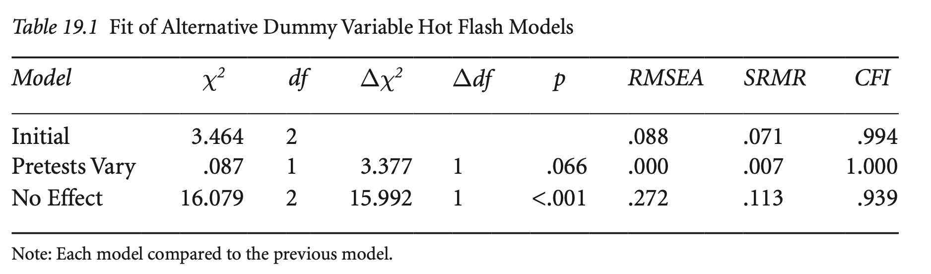
2 treatment 14.4 5.04 39 10.9모형에 대한 여러 가정들과 효과들을 검증
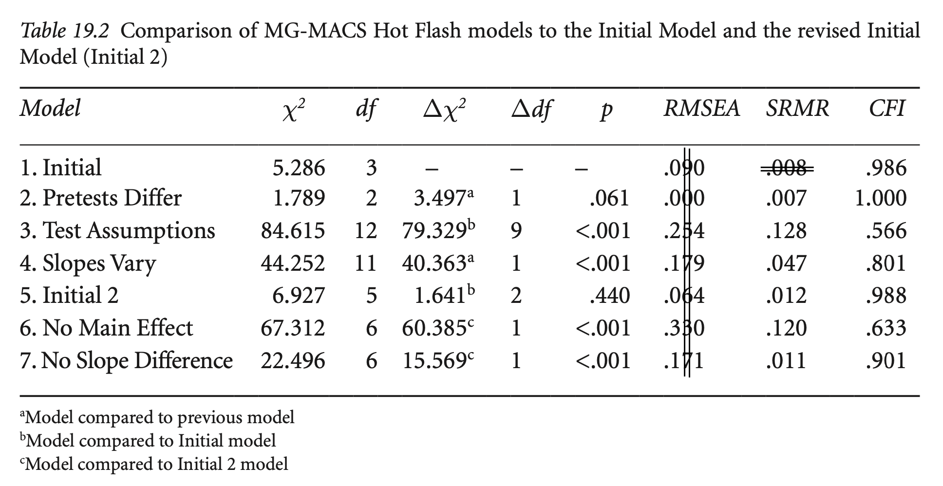
Keith’s Table 19.2에서 RMSEA값은 조정되지 않은 값으로 \(\sqrt{2}\)를 곱해야 lavaan/Mplus 결과값과 동일함.
사전 검사에서 두 집단 간의 평균(intercept)이 같다는 가정을 하지 않았을 때,
즉, free the estimate of the intercepts for the pretest latent variables
# free pretest intercepts
hotflash_model_mg2 <- "
  hf_pre =~ int1 + HF1
  hf_post =~ int2 + HF2

  hf_post ~ hf_pre

  HF1 ~~ HF2
  int1 ~~ int2

  # hf_pre ~ 0*1 # 제거
"
hotflash_fit_mg2 <- sem(hotflash_model_mg2,
  data = hotflash,
  meanstructure = TRUE,
  group = "g", # factor type
  group.equal = c("loadings", "intercepts")
)summary(hotflash_fit_mg2, estimates = FALSE) |> print()lavaan 0.6-19 ended normally after 316 iterations
Estimator ML
Optimization method NLMINB
Number of model parameters 32
Number of equality constraints 6
Number of observations per group:
control 48
treatment 48
Model Test User Model:
Test statistic 1.827
Degrees of freedom 2
P-value (Chi-square) 0.401
Test statistic for each group:
control 0.069
treatment 1.758parameterEstimates(hotflash_fit_mg2) |> subset(op == "~1") |> print() lhs op rhs block group label est se z pvalue ci.lower ci.upper
14 int1 ~1 1 1 .p14. 46.160 2.931 15.749 0.000 40.415 51.904
15 HF1 ~1 1 1 .p15. 17.176 1.460 11.763 0.000 14.315 20.038
16 int2 ~1 1 1 .p16. 42.265 3.128 13.513 0.000 36.135 48.395
17 HF2 ~1 1 1 .p17. 15.587 1.547 10.077 0.000 12.555 18.619
18 hf_pre ~1 1 1 0.000 0.000 NA NA 0.000 0.000
19 hf_post ~1 1 1 0.000 0.000 NA NA 0.000 0.000
33 int1 ~1 2 2 .p14. 46.160 2.931 15.749 0.000 40.415 51.904
34 HF1 ~1 2 2 .p15. 17.176 1.460 11.763 0.000 14.315 20.038
35 int2 ~1 2 2 .p16. 42.265 3.128 13.513 0.000 36.135 48.395
36 HF2 ~1 2 2 .p17. 15.587 1.547 10.077 0.000 12.555 18.619
37 hf_pre ~1 2 2 -6.970 3.653 -1.908 0.056 -14.131 0.190
38 hf_post ~1 2 2 -34.716 5.690 -6.101 0.000 -45.869 -23.564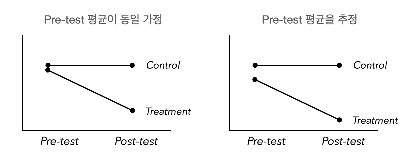
compareFit(hotflash_fit_mg, hotflash_fit_mg2) |> summary() |> print()################### Nested Model Comparison #########################
Chi-Squared Difference Test
Df AIC BIC Chisq Chisq diff RMSEA Df diff Pr(>Chisq)
hotflash_fit_mg2 2 2899.9 2966.6 1.8271
hotflash_fit_mg 3 2901.5 2965.6 5.3986 3.5715 0.23146 1 0.05878 .
---
Signif. codes: 0 ‘***’ 0.001 ‘**’ 0.01 ‘*’ 0.05 ‘.’ 0.1 ‘ ’ 1
####################### Model Fit Indices ###########################
chisq df pvalue rmsea cfi tli srmr aic bic
hotflash_fit_mg2 1.827† 2 .401 .000† 1.000† 1.006† .041† 2899.894† 2966.567
hotflash_fit_mg 5.399 3 .145 .129 .986 .944 .088 2901.465 2965.574†
################## Differences in Fit Indices #######################
df rmsea cfi tli srmr aic bic
hotflash_fit_mg - hotflash_fit_mg2 1 0.129 -0.014 -0.062 0.047 1.572 -0.993
The following lavaan models were compared:
hotflash_fit_mg2
hotflash_fit_mg
To view results, assign the compareFit() output to an object and use the summary() method; see the class?FitDiff help page.더미 변수 방식과 MG-MACS 방식의 비교
더미 변수 방식의 추정에서 숨은 가정들
이전 더미 변수 방식의 경우:
# Test assumptions
hotflash_model_mg3 <- "
  hf_pre =~ int1 + HF1
  hf_post =~ int2 + HF2

  hf_post ~ c(a, a)*hf_pre  # 사전 검사가 사후 검사에 동일하게 영향을 미친다고 가정

  HF1 ~~ HF2
  int1 ~~ int2

  hf_pre ~ 0*1  # pretest 동일성 가정
"
hotflash_fit_mg3 <- sem(hotflash_model_mg3,
  data = hotflash,
  meanstructure = TRUE,
  group = "g", # factor type
  group.equal = c(
    "loadings", "intercepts",
    "residuals", "lv.variances",
    "residual.covariances"
  )
)parameterEstimates(hotflash_fit_mg3) |> subset(op == "~") |> print() lhs op rhs block group label est se z pvalue ci.lower ci.upper
5 hf_post ~ hf_pre 1 1 a 0.487 0.195 2.5 0.012 0.105 0.868
24 hf_post ~ hf_pre 2 2 a 0.487 0.195 2.5 0.012 0.105 0.868parameterEstimates(hotflash_fit_mg3) |> subset(op == "~~") |> print() lhs op rhs block group label est se z pvalue ci.lower ci.upper
6 HF1 ~~ HF2 1 1 .p6. 60.277 10.820 5.571 0.000 39.071 81.484
7 int1 ~~ int2 1 1 .p7. -24.643 55.046 -0.448 0.654 -132.531 83.246
9 int1 ~~ int1 1 1 .p9. 52.755 179.207 0.294 0.768 -298.483 403.993
10 HF1 ~~ HF1 1 1 .p10. 98.604 17.851 5.524 0.000 63.617 133.592
11 int2 ~~ int2 1 1 .p11. 70.300 51.321 1.370 0.171 -30.286 170.887
12 HF2 ~~ HF2 1 1 .p12. 53.415 9.107 5.865 0.000 35.566 71.265
13 hf_pre ~~ hf_pre 1 1 .p13. 349.971 190.043 1.842 0.066 -22.507 722.449
14 hf_post ~~ hf_post 1 1 .p14. 138.752 35.569 3.901 0.000 69.039 208.465
25 HF1 ~~ HF2 2 2 .p6. 60.277 10.820 5.571 0.000 39.071 81.484
26 int1 ~~ int2 2 2 .p7. -24.643 55.046 -0.448 0.654 -132.531 83.246
28 int1 ~~ int1 2 2 .p9. 52.755 179.207 0.294 0.768 -298.483 403.993
29 HF1 ~~ HF1 2 2 .p10. 98.604 17.851 5.524 0.000 63.617 133.592
30 int2 ~~ int2 2 2 .p11. 70.300 51.321 1.370 0.171 -30.286 170.887
31 HF2 ~~ HF2 2 2 .p12. 53.415 9.107 5.865 0.000 35.566 71.265
32 hf_pre ~~ hf_pre 2 2 .p13. 349.971 190.043 1.842 0.066 -22.507 722.449
33 hf_post ~~ hf_post 2 2 .p14. 138.752 35.569 3.901 0.000 69.039 208.465parameterEstimates(hotflash_fit_mg3) |> subset(op == "~1") |> print() lhs op rhs block group label est se z pvalue ci.lower ci.upper
8 hf_pre ~1 1 1 0.000 0.000 NA NA 0.000 0.000
15 int1 ~1 1 1 .p15. 42.656 2.048 20.826 0 38.642 46.671
16 HF1 ~1 1 1 .p16. 15.737 1.128 13.949 0 13.525 17.948
17 int2 ~1 1 1 .p17. 40.870 2.349 17.396 0 36.266 45.475
18 HF2 ~1 1 1 .p18. 14.713 1.044 14.088 0 12.666 16.760
19 hf_post ~1 1 1 0.000 0.000 NA NA 0.000 0.000
27 hf_pre ~1 2 2 0.000 0.000 NA NA 0.000 0.000
34 int1 ~1 2 2 .p15. 42.656 2.048 20.826 0 38.642 46.671
35 HF1 ~1 2 2 .p16. 15.737 1.128 13.949 0 13.525 17.948
36 int2 ~1 2 2 .p17. 40.870 2.349 17.396 0 36.266 45.475
37 HF2 ~1 2 2 .p18. 14.713 1.044 14.088 0 12.666 16.760
38 hf_post ~1 2 2 -28.615 3.149 -9.087 0 -34.787 -22.444앞서 더미 변수 방식의 결과와 달리 모형 적합도가 매우 좋지 않음!
# Dummy 방식과의 비교
compareFit(hotflash_fit, hotflash_fit_mg3, nested = FALSE) |> summary() |> print()
####################### Model Fit Indices ###########################
chisq df pvalue rmsea cfi tli srmr aic bic
hotflash_fit 3.501† 2 .174 .088† .994† .968† .082† 2956.482† 2987.254†
hotflash_fit_mg3 86.416 12 .000 .359 .565 .565 .534 2964.482 3005.512
The following lavaan models were compared:
hotflash_fit
hotflash_fit_mg3
To view results, assign the compareFit() output to an object and use the summary() method; see the class?FitDiff help page.# Initial model과의 비교
compareFit(hotflash_fit_mg, hotflash_fit_mg3) |> summary()|> print()################### Nested Model Comparison #########################
Chi-Squared Difference Test
Df AIC BIC Chisq Chisq diff RMSEA Df diff Pr(>Chisq)
hotflash_fit_mg 3 2901.5 2965.6 5.3986
hotflash_fit_mg3 12 2964.5 3005.5 86.4155 81.017 0.4083 9 1.015e-13 ***
---
Signif. codes: 0 ‘***’ 0.001 ‘**’ 0.01 ‘*’ 0.05 ‘.’ 0.1 ‘ ’ 1
####################### Model Fit Indices ###########################
chisq df pvalue rmsea cfi tli srmr aic bic
hotflash_fit_mg 5.399† 3 .145 .129† .986† .944† .088† 2901.465† 2965.574†
hotflash_fit_mg3 86.416 12 .000 .359 .565 .565 .534 2964.482 3005.512
################## Differences in Fit Indices #######################
df rmsea cfi tli srmr aic bic
hotflash_fit_mg3 - hotflash_fit_mg 9 0.23 -0.421 -0.379 0.446 63.017 39.938
The following lavaan models were compared:
hotflash_fit_mg
hotflash_fit_mg3
To view results, assign the compareFit() output to an object and use the summary() method; see the class?FitDiff help page.앞의 모형에서 ANCOVA의 가정인 두 집단 간에 pre-test와 post-test의 관계가 동일하다는 가정을 검증함.
즉, 앞의 모든 가정을 포함한 모형에서, 집단 별로 기울기만 다르게 추정하면,
# Slopes Vary
hotflash_model_mg4 <- "
  hf_pre =~ int1 + HF1
  hf_post =~ int2 + HF2

  hf_post ~ c(a, b)*hf_pre

  HF1 ~~ HF2
  int1 ~~ int2

  hf_pre ~ 0*1
"
hotflash_fit_mg4 <- sem(hotflash_model_mg4,
  data = hotflash,
  meanstructure = TRUE,
  group = "g", # factor type
  group.equal = c(
    "loadings", "intercepts",
    "residuals", "lv.variances",
    "residual.covariances"
  )
)compareFit(hotflash_fit_mg3, hotflash_fit_mg4) |> summary() |> print()################### Nested Model Comparison #########################
Chi-Squared Difference Test
Df AIC BIC Chisq Chisq diff RMSEA Df diff Pr(>Chisq)
hotflash_fit_mg4 11 2925.3 2968.8 45.194
hotflash_fit_mg3 12 2964.5 3005.5 86.415 41.222 0.9154 1 1.359e-10 ***
---
Signif. codes: 0 ‘***’ 0.001 ‘**’ 0.01 ‘*’ 0.05 ‘.’ 0.1 ‘ ’ 1
####################### Model Fit Indices ###########################
chisq df pvalue rmsea cfi tli srmr aic bic
hotflash_fit_mg4 45.194† 11 .000 .254† .800† .782† .209† 2925.260† 2968.854†
hotflash_fit_mg3 86.416 12 .000 .359 .565 .565 .534 2964.482 3005.512
################## Differences in Fit Indices #######################
df rmsea cfi tli srmr aic bic
hotflash_fit_mg3 - hotflash_fit_mg4 1 0.105 -0.235 -0.217 0.325 39.222 36.658
The following lavaan models were compared:
hotflash_fit_mg4
hotflash_fit_mg3
To view results, assign the compareFit() output to an object and use the summary() method; see the class?FitDiff help page.Initial 모형의 적합도가 낮은 이유로 인해 더 나은 모형으로 개선
두 집단에서 모두 Cov(int1, int2)가 통계적으로 유의하지 않으므로 0으로 제약
Chi-square가 약간 증가하나 추가 자유도 2 확보
parameterEstimates(hotflash_fit_mg) |> subset(op == "~~") |> print() lhs op rhs block group label est se z pvalue ci.lower ci.upper
6 HF1 ~~ HF2 1 1 67.058 18.003 3.725 0.000 31.773 102.344
7 int1 ~~ int2 1 1 -28.916 98.630 -0.293 0.769 -222.227 164.396
9 int1 ~~ int1 1 1 170.287 124.805 1.364 0.172 -74.326 414.900
10 HF1 ~~ HF1 1 1 74.107 19.536 3.793 0.000 35.817 112.397
11 int2 ~~ int2 1 1 39.030 107.473 0.363 0.716 -171.614 249.674
12 HF2 ~~ HF2 1 1 81.674 19.666 4.153 0.000 43.128 120.220
13 hf_pre ~~ hf_pre 1 1 287.136 148.917 1.928 0.054 -4.735 579.008
14 hf_post ~~ hf_post 1 1 68.950 49.956 1.380 0.168 -28.962 166.863
25 HF1 ~~ HF2 2 2 47.191 10.578 4.461 0.000 26.460 67.923
26 int1 ~~ int2 2 2 44.760 37.540 1.192 0.233 -28.817 118.337
28 int1 ~~ int1 2 2 241.229 74.588 3.234 0.001 95.039 387.419
29 HF1 ~~ HF1 2 2 99.551 23.596 4.219 0.000 53.304 145.798
30 int2 ~~ int2 2 2 81.492 25.448 3.202 0.001 31.615 131.368
31 HF2 ~~ HF2 2 2 24.780 5.610 4.417 0.000 13.785 35.775
32 hf_pre ~~ hf_pre 2 2 114.255 70.087 1.630 0.103 -23.113 251.622
33 hf_post ~~ hf_post 2 2 2.901 52.283 0.055 0.956 -99.571 105.373# Initial 2: remove covariances between int1, int2
hotflash_model_mg5 <- "
hf_pre =~ int1 + HF1
hf_post =~ int2 + HF2
hf_post ~ hf_pre
HF1 ~~ HF2
int1 ~~ 0*int2 # fix the covariance to 0
hf_pre ~ 0*1
"
hotflash_fit_mg5 <- sem(hotflash_model_mg5,
data = hotflash,
meanstructure = TRUE,
group = "g", # factor type
group.equal = c("loadings", "intercepts")
)compareFit(hotflash_fit_mg, hotflash_fit_mg5) |> summary() |> print()################### Nested Model Comparison #########################
Chi-Squared Difference Test
Df AIC BIC Chisq Chisq diff RMSEA Df diff Pr(>Chisq)
hotflash_fit_mg 3 2901.5 2965.6 5.3986
hotflash_fit_mg5 5 2899.1 2958.1 7.0745 1.6759 0 2 0.4326
####################### Model Fit Indices ###########################
chisq df pvalue rmsea cfi tli srmr aic bic
hotflash_fit_mg 5.399† 3 .145 .129 .986 .944 .088† 2901.465 2965.574
hotflash_fit_mg5 7.074 5 .215 .093† .988† .971† .095 2899.141† 2958.121†
################## Differences in Fit Indices #######################
df rmsea cfi tli srmr aic bic
hotflash_fit_mg5 - hotflash_fit_mg 2 -0.036 0.002 0.027 0.006 -2.324 -7.453
The following lavaan models were compared:
hotflash_fit_mg
hotflash_fit_mg5
To view results, assign the compareFit() output to an object and use the summary() method; see the class?FitDiff help page.치료의 효과가 없다는 가정: post-test 잠재변수의 intercept를 0으로 제약
(pre-test 잠재변수의 intercept는 0으로 제약되어 있음)
# No main effect
hotflash_model_mg6 <- "
  hf_pre =~ int1 + HF1
  hf_post =~ int2 + HF2

  hf_post ~ hf_pre

  HF1 ~~ HF2
  int1 ~~ 0*int2  # fix the covariance to 0

  hf_pre ~ 0*1
  hf_post ~ 0*1  # fix the intercepts to 0 (아래 group.equal에서 means을 동일하게 제약하는 것과 같은 결과)
"
hotflash_fit_mg6 <- sem(hotflash_model_mg6,
  data = hotflash,
  meanstructure = TRUE,
  group = "g", # factor type
  group.equal = c("loadings", "intercepts",
                  "means") # fix the means to 0
)compareFit(hotflash_fit_mg5, hotflash_fit_mg6) |> summary() |> print()################### Nested Model Comparison #########################
Chi-Squared Difference Test
Df AIC BIC Chisq Chisq diff RMSEA Df diff Pr(>Chisq)
hotflash_fit_mg5 5 2899.1 2958.1 7.0745
hotflash_fit_mg6 6 2958.8 3015.2 68.7447 61.67 1.1243 1 4.061e-15 ***
---
Signif. codes: 0 ‘***’ 0.001 ‘**’ 0.01 ‘*’ 0.05 ‘.’ 0.1 ‘ ’ 1
####################### Model Fit Indices ###########################
chisq df pvalue rmsea cfi tli srmr aic bic
hotflash_fit_mg5 7.074† 5 .215 .093† .988† .971† .095† 2899.141† 2958.121†
hotflash_fit_mg6 68.745 6 .000 .467 .633 .266 .524 2958.811 3015.227
################## Differences in Fit Indices #######################
df rmsea cfi tli srmr aic bic
hotflash_fit_mg6 - hotflash_fit_mg5 1 0.374 -0.355 -0.705 0.429 59.67 57.106
The following lavaan models were compared:
hotflash_fit_mg5
hotflash_fit_mg6
To view results, assign the compareFit() output to an object and use the summary() method; see the class?FitDiff help page.parameterEstimates(hotflash_fit_mg5, standardized = "std.all") |> subset(op == "~1" & lhs == "hf_post") |> print() lhs op rhs block group label est se z pvalue ci.lower ci.upper std.all
19 hf_post ~1 1 1 0.000 0.000 NA NA 0.000 0.000 0.00
38 hf_post ~1 2 2 -28.308 3.143 -9.006 0 -34.468 -22.147 -4.25두 모형의 큰 차이는 chi-square difference test에서나 post-test의 intercept에 대한 유의성 테스트에서나 동일하게 나타남.
치료 효과의 크기에 대해서는 Int 변수의 metric으로 28.3점 감소한다고 해석할 수 있으나, 표준화하려면 Pre-test의 통제집단과 처치집단의 pooled standard deviation을 사용해야 함; 여러 방식이 제안됨. 논란의 여지가 있음! 참고
즉, cohen’s d = -28.3 / pooled SD = \(\displaystyle \frac{-28.3}{\sqrt{\frac{255.7 + 143.7}{2}}} = -2.00\)
앞서 더미 변수 방식에서는 Group(Hypnosis) → Post의 회귀계수는 -28.6(비표준화), -1.39(표준화)
Latent Change Score Model 방식도 고려; 맨 아래
# Pre-test 잠재변수의 분산 확인
parameterEstimates(hotflash_fit_mg5) |> subset(op == "~~" & (lhs == "hf_pre")) |> print()
lhs op rhs block group label est se z pvalue ci.lower ci.upper
13 hf_pre ~~ hf_pre 1 1 255.650 97.491 2.622 0.009 64.572 446.727
32 hf_pre ~~ hf_pre 2 2 143.736 60.058 2.393 0.017 26.024 261.449parameterEstimates(hotflash_fit_mg5) |> subset(op == "~~") |> print() lhs op rhs block group label est se z pvalue ci.lower ci.upper
6 HF1 ~~ HF2 1 1 64.439 15.850 4.066 0.000 33.373 95.505
7 int1 ~~ int2 1 1 0.000 0.000 NA NA 0.000 0.000
9 int1 ~~ int1 1 1 200.813 65.273 3.076 0.002 72.880 328.747
10 HF1 ~~ HF1 1 1 70.829 16.758 4.226 0.000 37.983 103.674
11 int2 ~~ int2 1 1 62.914 75.243 0.836 0.403 -84.560 210.388
12 HF2 ~~ HF2 1 1 79.187 17.862 4.433 0.000 44.179 114.196
13 hf_pre ~~ hf_pre 1 1 255.650 97.491 2.622 0.009 64.572 446.727
14 hf_post ~~ hf_post 1 1 70.303 49.163 1.430 0.153 -26.054 166.660
25 HF1 ~~ HF2 2 2 46.821 10.332 4.532 0.000 26.571 67.072
26 int1 ~~ int2 2 2 0.000 0.000 NA NA 0.000 0.000
28 int1 ~~ int1 2 2 206.182 65.952 3.126 0.002 76.918 335.447
29 HF1 ~~ HF1 2 2 96.979 23.606 4.108 0.000 50.712 143.247
30 int2 ~~ int2 2 2 68.308 20.877 3.272 0.001 27.389 109.227
31 HF2 ~~ HF2 2 2 23.690 5.445 4.351 0.000 13.018 34.362
32 hf_pre ~~ hf_pre 2 2 143.736 60.058 2.393 0.017 26.024 261.449
33 hf_post ~~ hf_post 2 2 39.097 22.874 1.709 0.087 -5.735 83.930앞서 Slopes differs에서처럼 pretest → posttest의 관계가 집단에 따라 동일하다고 가정하면,
즉, no slope difference를 가정
# No slope difference: interaction
hotflash_model_mg7 <- "
  hf_pre =~ int1 + HF1
  hf_post =~ int2 + HF2

  hf_post ~ c(a, a)*hf_pre

  HF1 ~~ HF2
  int1 ~~ 0*int2  # fix the covariance to 0

  hf_pre ~ 0*1
"
hotflash_fit_mg7 <- sem(hotflash_model_mg7,
  data = hotflash,
  meanstructure = TRUE,
  group = "g", # factor type
  group.equal = c("loadings", "intercepts")
)compareFit(hotflash_fit_mg5, hotflash_fit_mg7) |> summary() |> print()################### Nested Model Comparison #########################
Chi-Squared Difference Test
Df AIC BIC Chisq Chisq diff RMSEA Df diff Pr(>Chisq)
hotflash_fit_mg5 5 2899.1 2958.1 7.0745
hotflash_fit_mg7 6 2913.0 2969.5 22.9747 15.9 0.55716 1 6.677e-05 ***
---
Signif. codes: 0 ‘***’ 0.001 ‘**’ 0.01 ‘*’ 0.05 ‘.’ 0.1 ‘ ’ 1
####################### Model Fit Indices ###########################
chisq df pvalue rmsea cfi tli srmr aic bic
hotflash_fit_mg5 7.074† 5 .215 .093† .988† .971† .095† 2899.141† 2958.121†
hotflash_fit_mg7 22.975 6 .001 .243 .901 .801 .113 2913.041 2969.457
################## Differences in Fit Indices #######################
df rmsea cfi tli srmr aic bic
hotflash_fit_mg7 - hotflash_fit_mg5 1 0.15 -0.087 -0.169 0.018 13.9 11.336
The following lavaan models were compared:
hotflash_fit_mg5
hotflash_fit_mg7
To view results, assign the compareFit() output to an object and use the summary() method; see the class?FitDiff help page.parameterEstimates(hotflash_fit_mg5, standardized="std.all") |> subset(op == "~") |> print() lhs op rhs block group label est se z pvalue ci.lower ci.upper
5 hf_post ~ hf_pre 1 1 1.169 0.271 4.315 0.000 0.638 1.700
24 hf_post ~ hf_pre 2 2 -0.191 0.197 -0.972 0.331 -0.577 0.195
std.all
5 0.912
24 -0.345통제집단에서만 사전검사에서 높은 열감을 보고한 여성이 사후검사도 높은 열감을 보이는 상관관계(0.912)를 보임.
치료집단에서는 사전검사 수치가 사후검사에 영향을 주지 않는 것으로 보임.
즉, 사전검사와 어느 집단에 속하는지가 서로 상호작용하여 사후검사에 효과가 나타났음; interaction effect
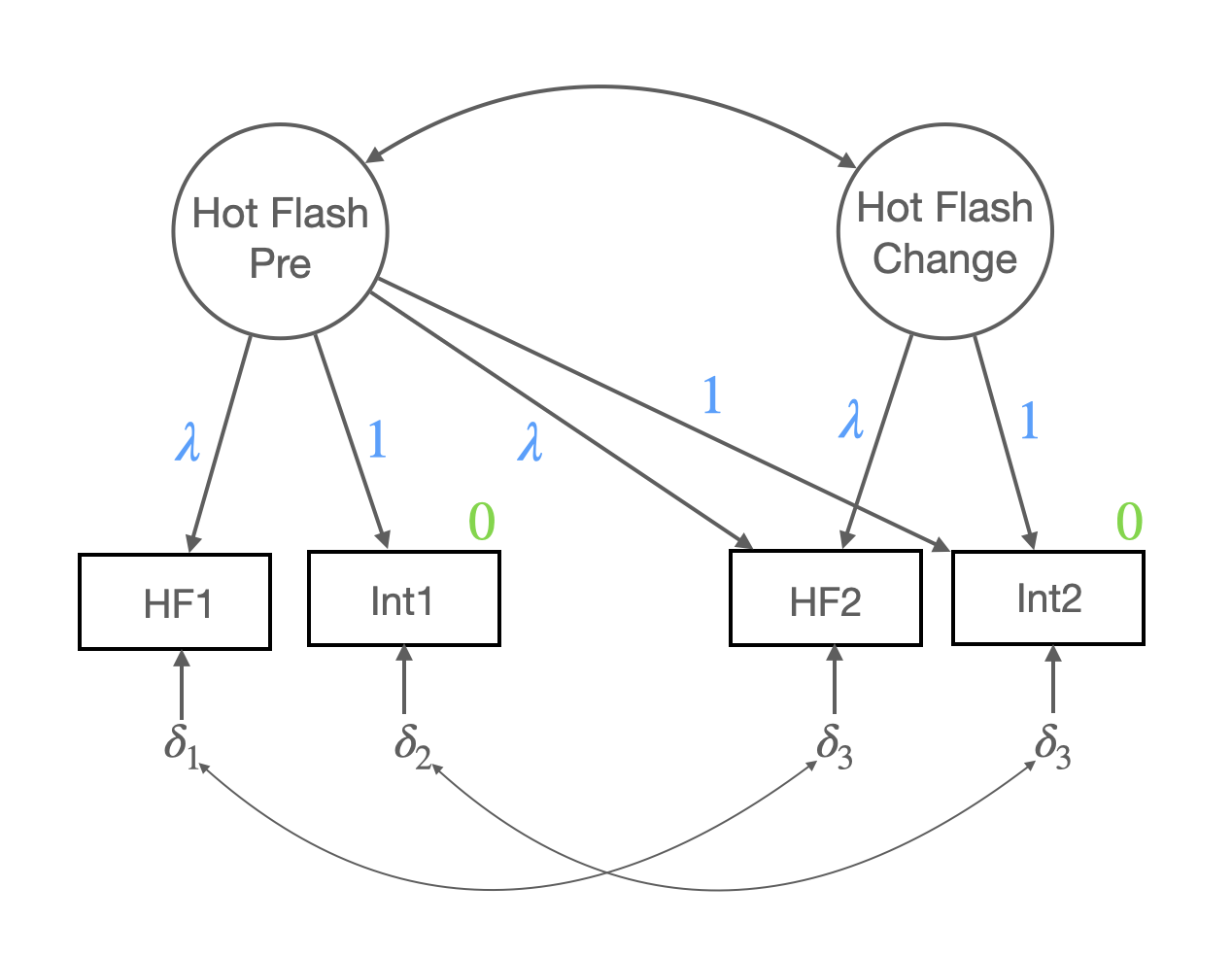
hotflash_model_mg_lcm <- "
  PreTest =~ 1*int1 + a*HF1 + 1*int2 + a*HF2
  Change =~ 1*int2 + a*HF2

  Change ~~ PreTest
  # Change ~~ c(d1, d1)*PreTest  # check the interaction effect

  HF1 ~~ HF2
  int1 ~~ 0*int2

  PreTest ~ 1
  Change ~ 1
  # Change ~ c(c1, c1)*1  # check the main effect
  int1 ~ 0*1
  int2 ~ 0*1
"
hotflash_fit_mg_lcm <- sem(hotflash_model_mg_lcm,
data = hotflash,
meanstructure = TRUE,
group = "g", # factor type
group.equal = c("loadings", "intercepts")
)
summary(hotflash_fit_mg_lcm,
standardized = TRUE,
fit.measures = TRUE,
remove.unused = FALSE, # keep the unused parameters
) |> print()lavaan 0.6-19 ended normally after 295 iterations
Estimator ML
Optimization method NLMINB
Number of model parameters 30
Number of equality constraints 7
Number of observations per group:
control 48
treatment 48
Model Test User Model:
Test statistic 4.325
Degrees of freedom 5
P-value (Chi-square) 0.504
Test statistic for each group:
control 0.602
treatment 3.723
Model Test Baseline Model:
Test statistic 182.941
Degrees of freedom 12
P-value 0.000
User Model versus Baseline Model:
Comparative Fit Index (CFI) 1.000
Tucker-Lewis Index (TLI) 1.009
Loglikelihood and Information Criteria:
Loglikelihood user model (H0) -1425.196
Loglikelihood unrestricted model (H1) -1423.033
Akaike (AIC) 2896.392
Bayesian (BIC) 2955.372
Sample-size adjusted Bayesian (SABIC) 2882.751
Root Mean Square Error of Approximation:
RMSEA 0.000
90 Percent confidence interval - lower 0.000
90 Percent confidence interval - upper 0.186
P-value H_0: RMSEA <= 0.050 0.571
P-value H_0: RMSEA >= 0.080 0.339
Standardized Root Mean Square Residual:
SRMR 0.067
Parameter Estimates:
Standard errors Standard
Information Expected
Information saturated (h1) model Structured
Group 1 [control]:
Latent Variables:
Estimate Std.Err z-value P(>|z|) Std.lv Std.all
PreTest =~
int1 1.000 17.587 0.814
HF1 (a) 0.344 0.038 9.047 0.000 6.044 0.579
int2 1.000 17.587 0.818
HF2 (a) 0.344 0.038 9.047 0.000 6.044 0.557
Change =~
int2 1.000 7.544 0.351
HF2 (a) 0.344 0.038 9.047 0.000 2.592 0.239
Covariances:
Estimate Std.Err z-value P(>|z|) Std.lv Std.all
PreTest ~~
Change -9.541 44.450 -0.215 0.830 -0.072 -0.072
.HF1 ~~
.HF2 63.485 15.644 4.058 0.000 63.485 0.852
.int1 ~~
.int2 0.000 0.000 0.000
Intercepts:
Estimate Std.Err z-value P(>|z|) Std.lv Std.all
PreTest 46.526 3.055 15.232 0.000 2.645 2.645
Change -4.518 2.470 -1.829 0.067 -0.599 -0.599
.int1 0.000 0.000 0.000
.int2 0.000 0.000 0.000
.HF1 (.20.) 1.191 1.705 0.698 0.485 1.191 0.114
.HF2 (.21.) 1.290 0.886 1.456 0.145 1.290 0.119
Variances:
Estimate Std.Err z-value P(>|z|) Std.lv Std.all
.int1 157.929 59.157 2.670 0.008 157.929 0.338
.HF1 72.423 16.558 4.374 0.000 72.423 0.665
.int2 114.843 57.030 2.014 0.044 114.843 0.249
.HF2 76.628 17.446 4.392 0.000 76.628 0.651
PreTest 309.313 85.946 3.599 0.000 1.000 1.000
Change 56.909 42.216 1.348 0.178 1.000 1.000
Group 2 [treatment]:
Latent Variables:
Estimate Std.Err z-value P(>|z|) Std.lv Std.all
PreTest =~
int1 1.000 12.867 0.701
HF1 (a) 0.344 0.038 9.047 0.000 4.422 0.400
int2 1.000 12.867 1.212
HF2 (a) 0.344 0.038 9.047 0.000 4.422 0.826
Change =~
int2 1.000 15.974 1.504
HF2 (a) 0.344 0.038 9.047 0.000 5.489 1.026
Covariances:
Estimate Std.Err z-value P(>|z|) Std.lv Std.all
PreTest ~~
Change -188.179 62.743 -2.999 0.003 -0.916 -0.916
.HF1 ~~
.HF2 46.707 10.353 4.512 0.000 46.707 0.954
.int1 ~~
.int2 0.000 0.000 0.000
Intercepts:
Estimate Std.Err z-value P(>|z|) Std.lv Std.all
PreTest 38.768 2.558 15.158 0.000 3.013 3.013
Change -27.749 3.103 -8.941 0.000 -1.737 -1.737
.int1 0.000 0.000 0.000
.int2 0.000 0.000 0.000
.HF1 (.20.) 1.191 1.705 0.698 0.485 1.191 0.108
.HF2 (.21.) 1.290 0.886 1.456 0.145 1.290 0.241
Variances:
Estimate Std.Err z-value P(>|z|) Std.lv Std.all
.int1 171.170 64.030 2.673 0.008 171.170 0.508
.HF1 102.362 23.079 4.435 0.000 102.362 0.840
.int2 68.417 19.755 3.463 0.001 68.417 0.607
.HF2 23.405 5.491 4.262 0.000 23.405 0.817
PreTest 165.561 63.980 2.588 0.010 1.000 1.000
Change 255.157 74.217 3.438 0.001 1.000 1.000
두 indicator의 metric을 고르게 반영하려면 effect coding을 고려해 볼 것.
hotflash_model_mg_lcm2 <- "
  PreTest =~ NA*b*HF1 + a*int1 + b*HF2 + a*int2
  Change =~ NA*b*HF2 + a*int2
  a + b == 2  # average loading = 1

  Change ~~ PreTest

  HF1 ~~ HF2
  int1 ~~ 0*int2

  PreTest ~ 1
  Change ~ 1

  HF1 ~ c1*1
  int1 ~ c2*1
  c1 + c2 == 0  # average intercept = 0

  HF2 ~ d1*1
  int2 ~ d2*1
  d1 + d2 == 0  # average intercept = 0
"
hotflash_fit_mg_lcm2 <- sem(hotflash_model_mg_lcm2,
data = hotflash,
meanstructure = TRUE,
group = "g", # factor type
group.equal = c("loadings", "intercepts")
)
parameterEstimates(hotflash_fit_mg_lcm2) |> subset(op == "~1") |> print() lhs op rhs block group label est se z pvalue ci.lower ci.upper
10 PreTest ~1 1 1 31.853 2.015 15.811 0.000 27.905 35.802
11 Change ~1 1 1 -2.986 1.398 -2.136 0.033 -5.725 -0.247
12 HF1 ~1 1 1 c1 0.886 1.289 0.687 0.492 -1.641 3.413
13 int1 ~1 1 1 c2 -0.886 1.289 -0.687 0.492 -3.413 1.641
14 HF2 ~1 1 1 d1 0.960 0.678 1.416 0.157 -0.369 2.290
15 int2 ~1 1 1 d2 -0.960 0.678 -1.416 0.157 -2.290 0.369
31 PreTest ~1 2 2 26.641 1.714 15.545 0.000 23.282 30.000
32 Change ~1 2 2 -18.593 1.942 -9.574 0.000 -22.400 -14.787
33 HF1 ~1 2 2 c1 0.886 1.289 0.687 0.492 -1.641 3.413
34 int1 ~1 2 2 c2 -0.886 1.289 -0.687 0.492 -3.413 1.641
35 HF2 ~1 2 2 d1 0.960 0.678 1.416 0.157 -0.369 2.290
36 int2 ~1 2 2 d2 -0.960 0.678 -1.416 0.157 -2.290 0.369standardizedSolution(hotflash_fit_mg_lcm2) |> subset(op == "~1") |> print() lhs op rhs group label est.std se z pvalue ci.lower ci.upper
10 PreTest ~1 1 2.696 0.407 6.617 0.000 1.897 3.494
11 Change ~1 1 -0.589 0.355 -1.659 0.097 -1.285 0.107
12 HF1 ~1 1 c1 0.085 0.125 0.677 0.498 -0.161 0.331
13 int1 ~1 1 c2 -0.041 0.060 -0.688 0.491 -0.158 0.076
14 HF2 ~1 1 d1 0.089 0.064 1.373 0.170 -0.038 0.215
15 int2 ~1 1 d2 -0.045 0.032 -1.408 0.159 -0.107 0.018
31 PreTest ~1 2 3.082 0.601 5.132 0.000 1.905 4.259
32 Change ~1 2 -1.733 0.292 -5.934 0.000 -2.305 -1.160
33 HF1 ~1 2 c1 0.080 0.117 0.686 0.492 -0.149 0.309
34 int1 ~1 2 c2 -0.048 0.070 -0.686 0.493 -0.186 0.090
35 HF2 ~1 2 d1 0.179 0.128 1.404 0.160 -0.071 0.430
36 int2 ~1 2 d2 -0.090 0.065 -1.402 0.161 -0.217 0.036실제 평균값을 살펴보면,
hotflash <- hotflash |>
  mutate(hf_change = HF2 - HF1, int_change = int2 - int1)
hotflash |>
group_by(g) |>
summarise(across(HF1:int_change, mean)) |> print()# A tibble: 2 × 7
g HF1 HF2 int1 int2 hf_change int_change
<fct> <dbl> <dbl> <dbl> <dbl> <dbl> <dbl>
1 control 17.1 15.5 46.3 42.2 -1.57 -4.06
2 treatment 14.4 5.04 39 10.9 -9.36 -28.1